
Vector Databases Intuitively Explained
Learn the fundamentals of vector databases and how they enable advanced AI applications

What is a Vector Database?
A vector database is a database that stores information as vectors, which are numerical representations of data objects, also known as vector embedding- Elastic.co
VectorDB uses the power of vector embeddings to index and search across a massive dataset of unstructured data and semi-structured data, such as images, text, or sensor data. With a Vector Database, you can efficiently store and retrieve similar or related content for a query search. This makes it a powerful tool for processing and analyzing large volumes of text.
Where is VectorDB Used?
Vector databases are transforming how we search for information by enabling more advanced and accurate searches. They are also being used along with large language models to add external or private data to reduce hallucinations in LLM better. Some of the prominent use cases for VectorDB are,
Search Engines: Traditional search engines depend on keywords, which can miss the deeper/actual meaning of a query. Vector databases improve retrieval by converting text into vectors that capture its meaning, enabling us to get search results using semantic searching.
Recommender Systems: Vector databases are used for recommendation systems in companies like Netflix and Amazon. They use Approximate Nearest Neighbor (ANN) search to quickly find items similar to those users have liked, resulting in more personalized recommendations.
Large Language Models (LLMs) using the RAG framework: RAG systems today rely on Vector DB for pulling in external information from a custom/private knowledge base. Vector databases store and retrieve the relevant document content efficiently, supporting applications like chatbots.
When are Vector Databases Used in LLM Applications?
In many LLM applications, Vector Databases are used when the LLM itself doesn’t have all the information it needs. For instance, LLMs would not know about:
Very recent information: For example, news articles, recent technological advancements, or any content created after the LLM was last trained.
Private or confidential data: Personal information, internal company documents, or any other non-public data.
Because of these drawbacks with LLM, enterprises are exploring many RAG-based LLM applications for production apps, which use Vector Databases rather than vanilla LLM applications. Essentially, Vector Databases augment the LLM’s knowledge with up-to-date and private/ proprietary information, allowing it to provide more accurate and relevant responses.
How does Vector DB work?
A vector database could be imagined as an intelligent system that organizes data in a unique way, making it easy to find what you need. This is done using something called “vector embeddings,” which are like special machine-understandable codes that represent the meaning of the content stored in the database.
Step 1: Creating Embeddings
First, the database transforms content (text, images, audio, or video) into vector embeddings. This could be thought of as turning words into machine-understandable codes, which are then plotted as points on a map.
Step 2: Indexing
Next, it organizes these vector points using embedding models. The algorithms used in the Embedding models ensure that everything is mapped out so that similar text chunks/contents are positioned together, which allows for faster and more efficient searches.
Step 3: Querying
When you search for something, it converts your query to embeddings and compares it to the stored vector embeddings. It looks for the closest matches and then shows you the most relevant results.
In essence, a vector database works by converting content into searchable codes(create embeddings), organizing them efficiently(indexing), and then quickly finding the best matches(querying/retrieval) when you need information.
So, What Are Embeddings?
If you ask someone how they understand the meaning of words, they might need help to explain it. They “know” that “child” and “kid” mean the same thing; “red” and “green” are both colours and “pleased,” “happy,” and “elated” express similar emotions with different intensities. This understanding is deeply ingrained in our brains, even if we can’t articulate how it works.
Language models, like those used in AI, have a similar understanding of language, but instead of neurons and thoughts, they use numbers. In a language model, any human language can be represented as a vector — a list of numbers. This vector is called an embedding.
A key component of language models is the ability to convert human language into these numerical embeddings. Think of it as a “translator” that turns words into numbers. While we don’t fully understand what these numbers mean, the AI does. What’s fascinating is that similar words generate similar sets of numbers. This allows the AI to “understand” and “process” language in its way, even if that understanding is beyond our comprehension.
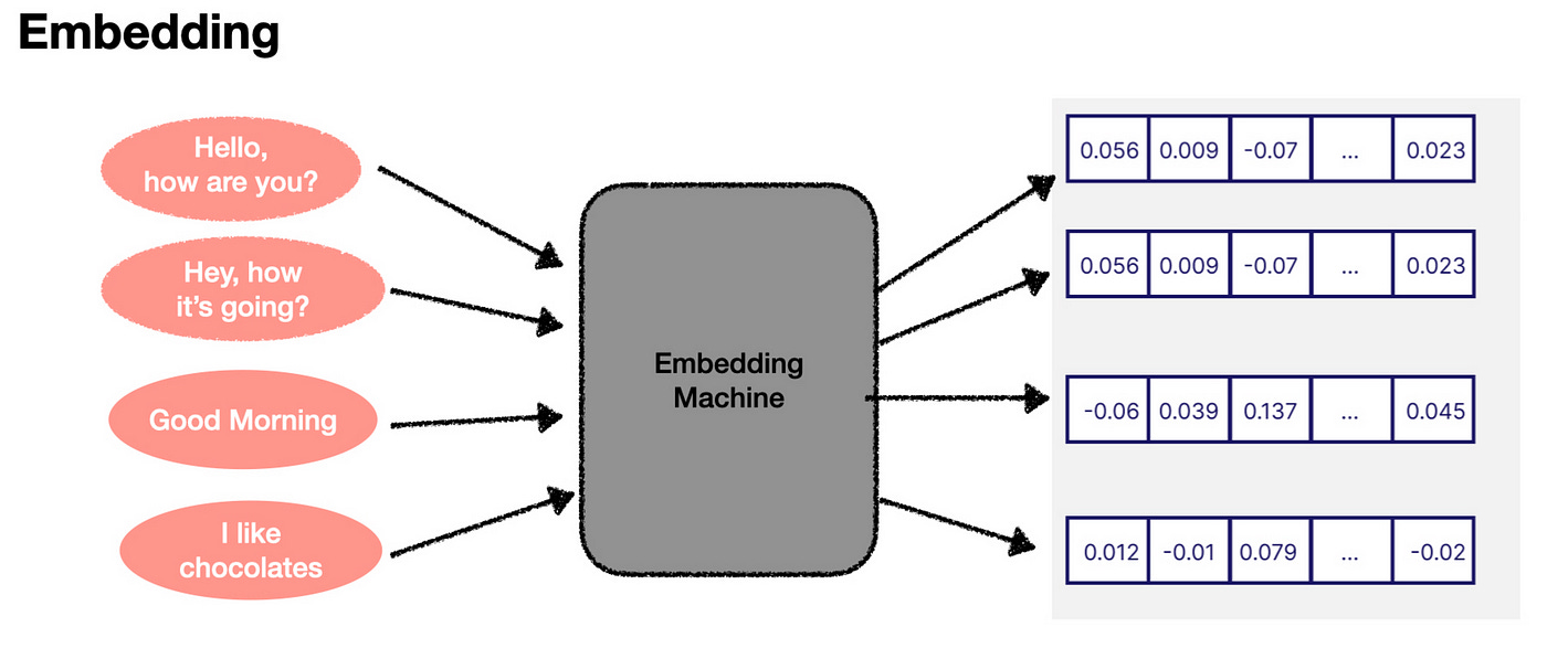
Now, these embeddings can be visualized in a conceptual space. Imagine plotting these numbers on a graph. If two words or phrases have similar meanings, their points on the graph will be close to each other. For example, “Hello, how are you?” and “Hey, how’s it going?” would be almost on top of each other, while “I like cupcakes” would be far away from these greetings.
In reality, embeddings exist in a much more complex, multi-dimensional space (1,536 dimensions in some models). But the basic idea is the same. The closer the two embeddings are, the more similar the pieces of text they represent. This concept is the foundation of semantic search, which is crucial for the retrieval process in AI systems. By comparing embeddings, the AI can determine which information most relates to a user’s query, enabling effective knowledge retrieval.
Enjoying the blog so far? Please subscribe to my substack to get similar insightful content directly to your inbox
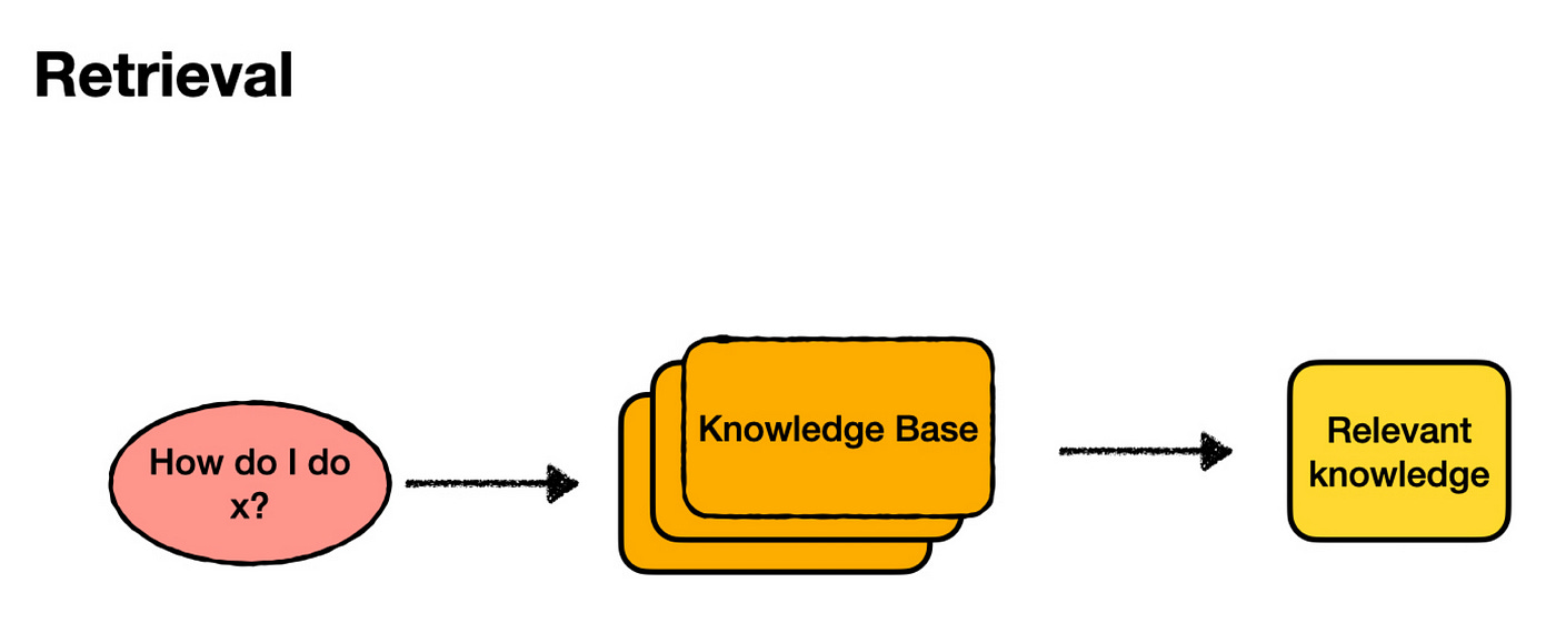
To understand how embeddings help in search, let’s break down the retrieval process.
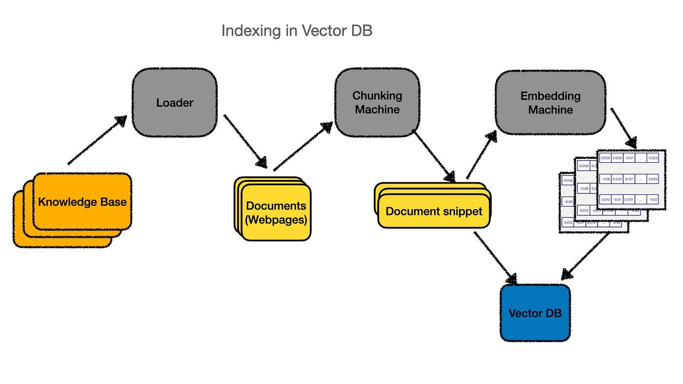
Indexing:
First, we need to divide our knowledge base into smaller chunks of text. This step involves some optimization, which we’ll explore later. For now, let’s assume we know how to do it.
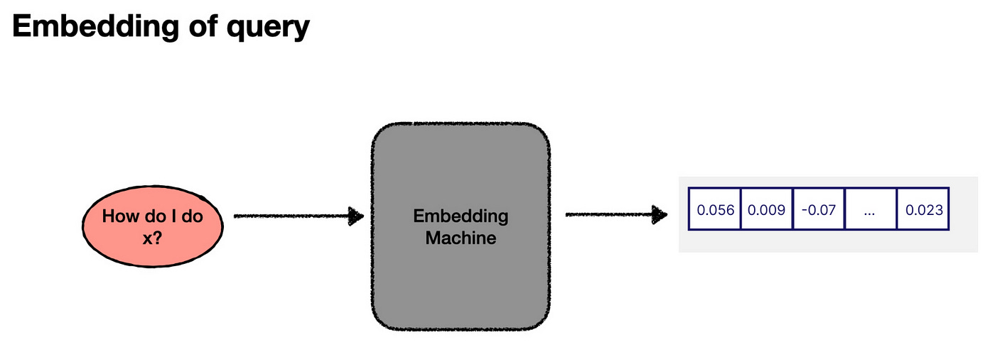
Once we’ve divided the text, each chunk is passed through an “embedding machine” (like an OpenAI API), which converts the text into an embedding — a numerical representation. We then store both the text snippet and its embedding in a vector database — a database specifically designed to handle these numerical vectors.
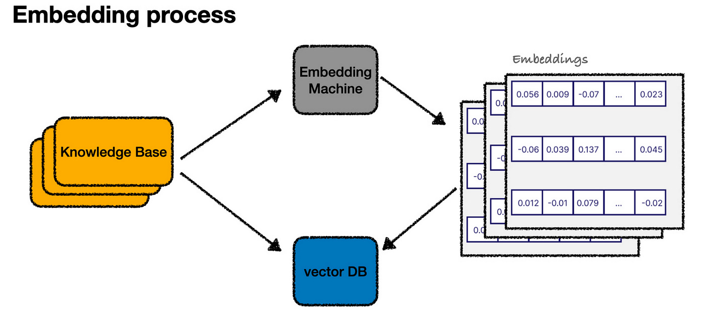
With all the content now represented as embeddings in our vector database, you can imagine it as a graph plotting our entire knowledge base in a “language” space.
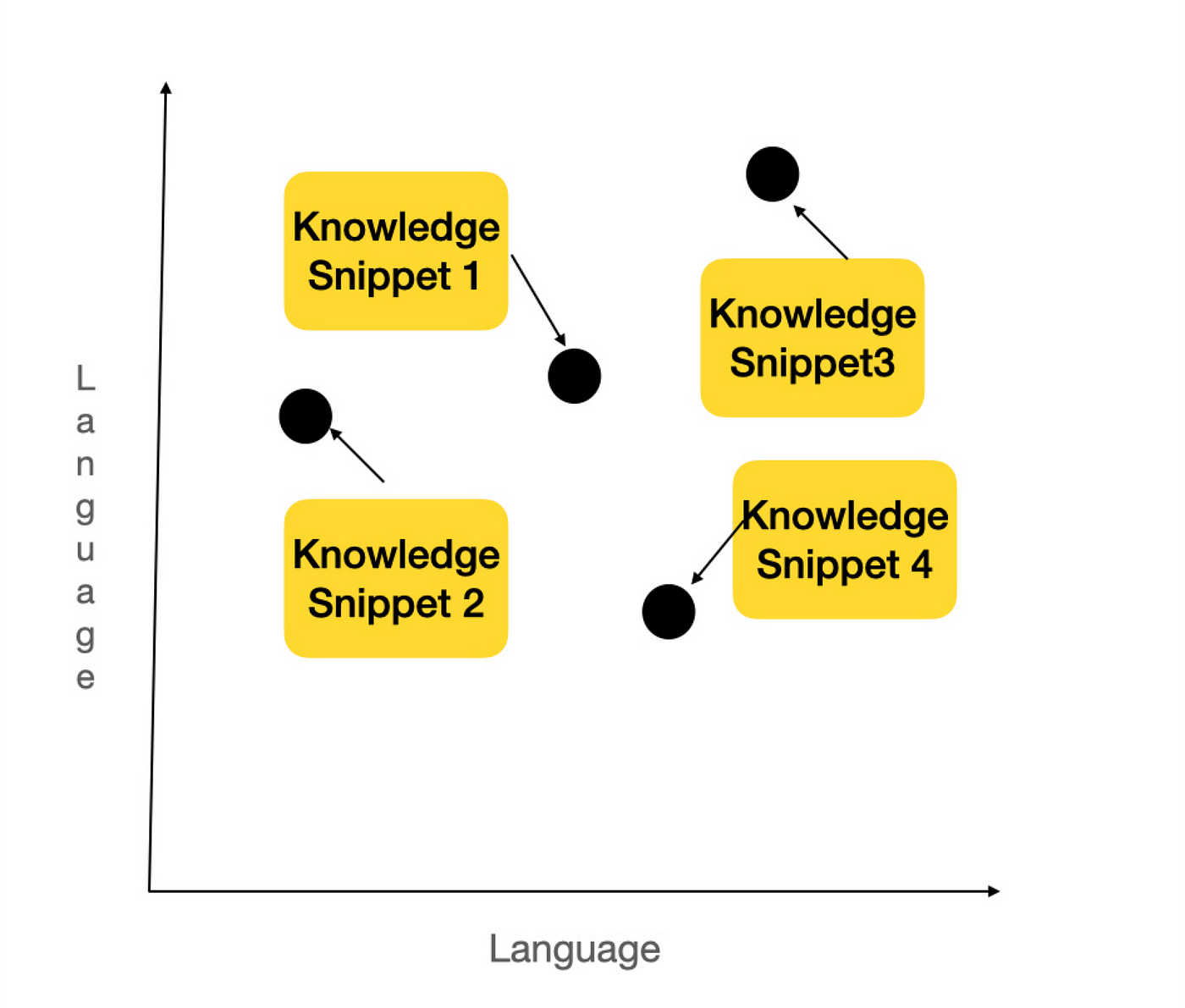
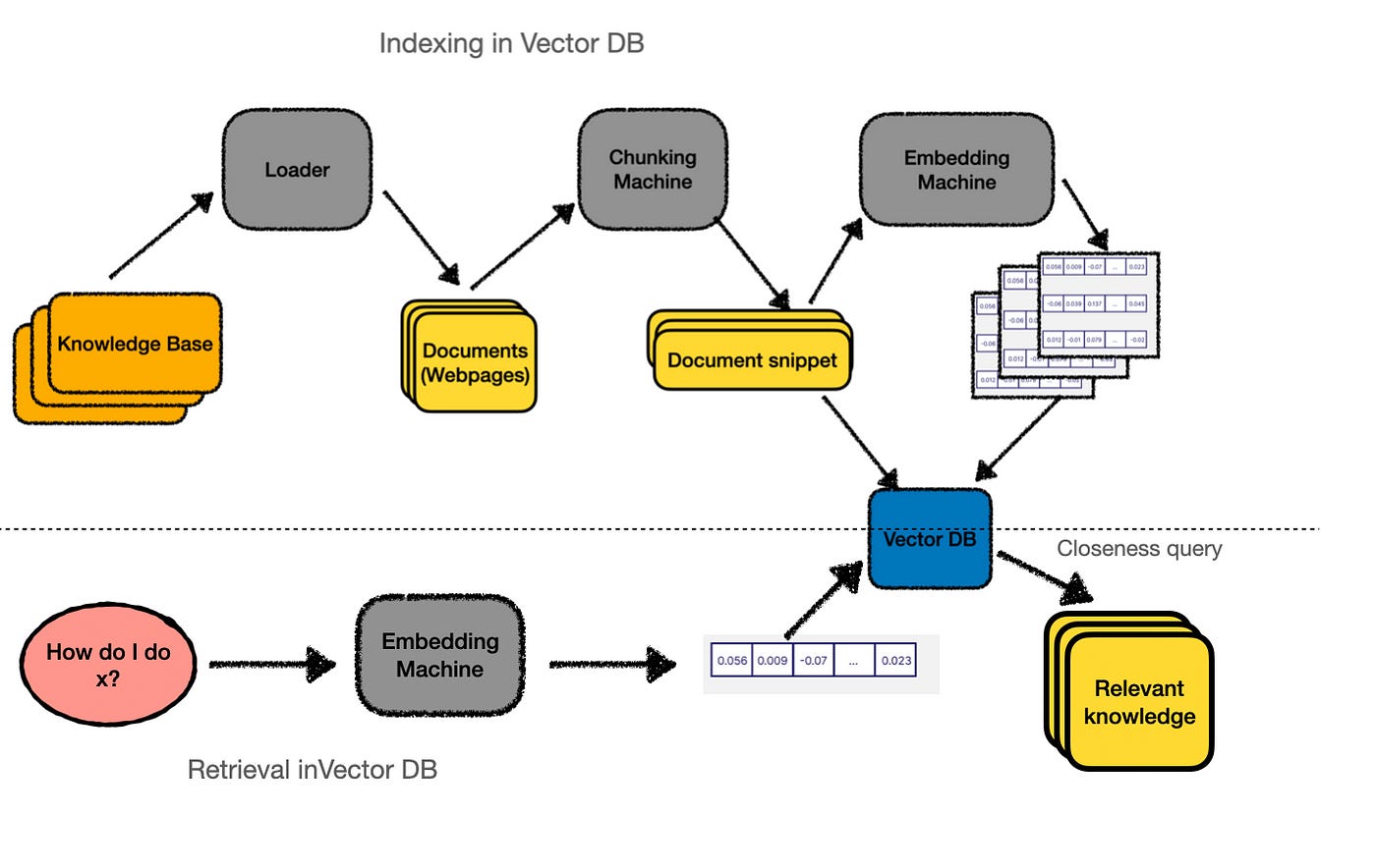
Querying:
When a user asks a question, we follow a similar process. We generate an embedding for the user’s input.
Then plot it in the same vector space, and then find the snippets that are closest to it (in this case, let’s say snippets 1 and 2).
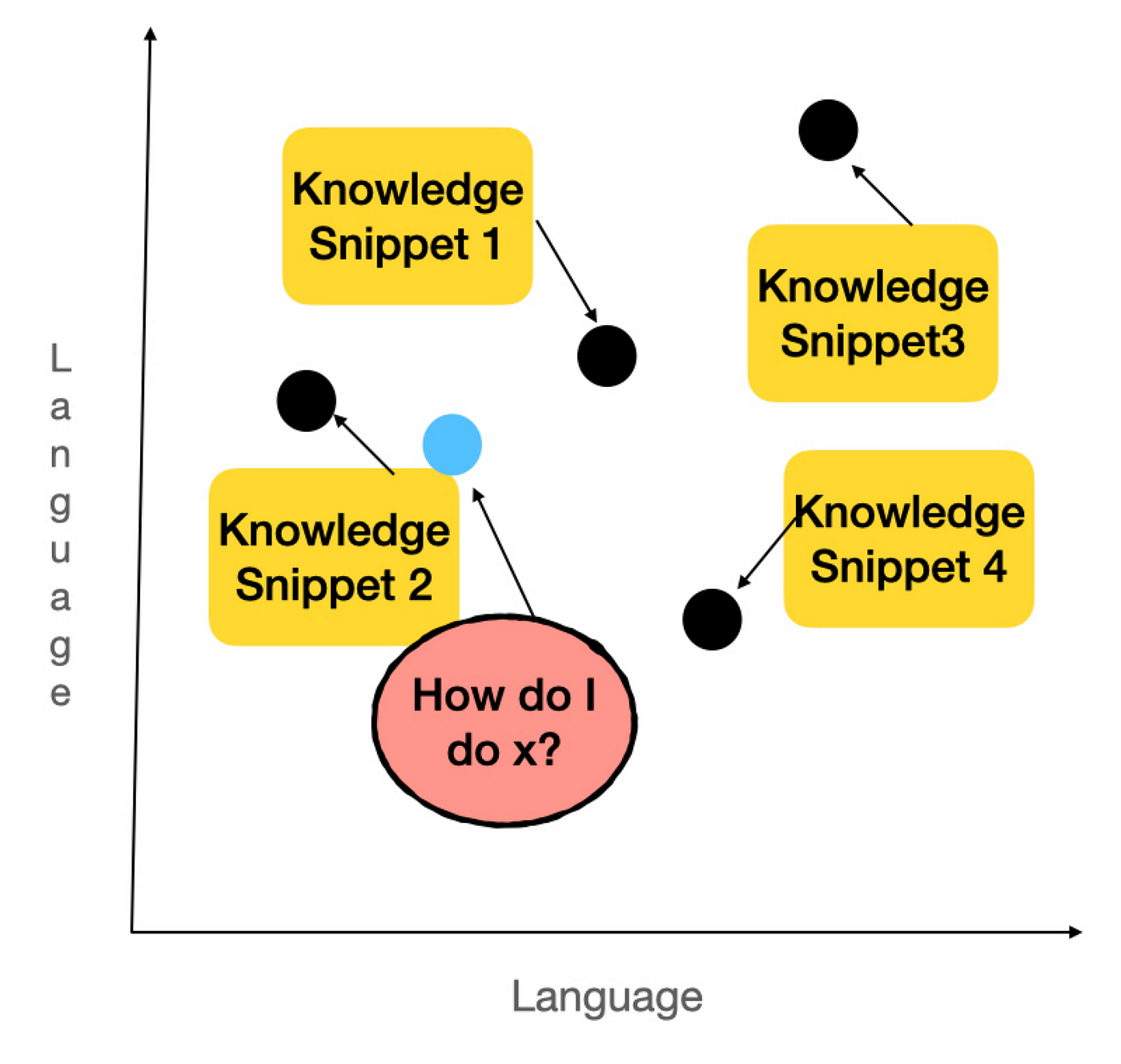
The embedding machine identifies these snippets as the most relevant answers to the user’s question, and we retrieve them to send to the LLM.
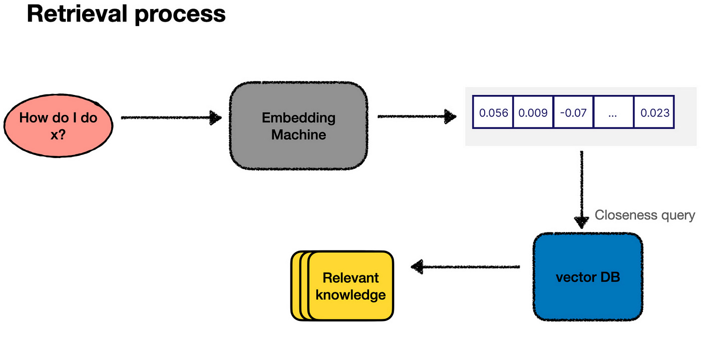
In practice, this process — finding the closest points — is performed by querying our vector database. So, the actual workflow looks more like this:
How do we index our data?
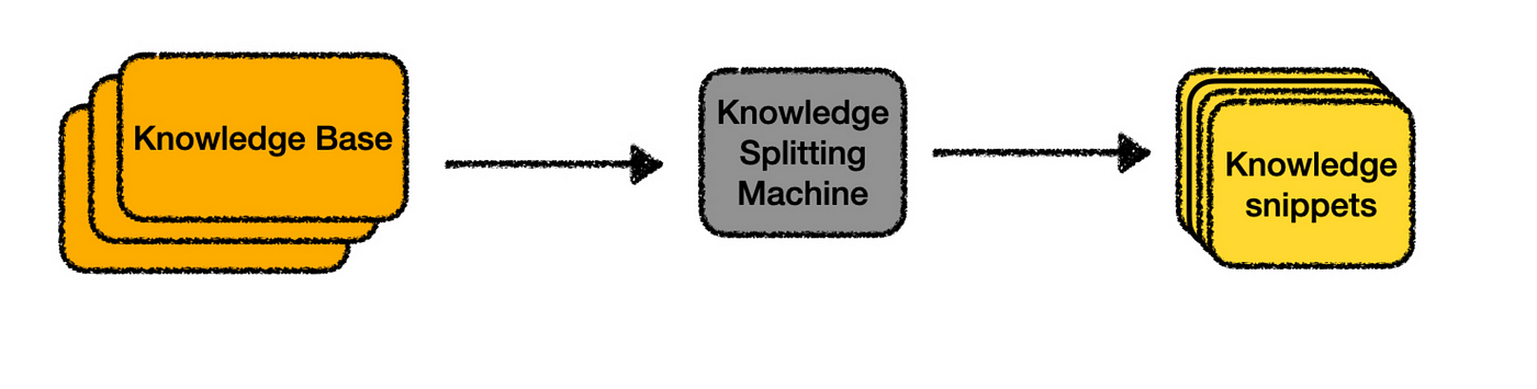
Now that we understand how embeddings can help us find the most relevant parts of our knowledge base and use them to get augmented answers from an LLM, the final step is creating that initial index from your knowledge base. In other words, we need to build the “knowledge-splitting machine.”
Surprisingly, indexing your knowledge base is often the most complex and crucial part of the entire process. It’s more of an art than a science and requires a lot of trial and error.
The indexing process can be broken down into two main steps:
1. Loading: Extracting the contents of your knowledge base from wherever it’s stored.
2. Splitting: Dividing the knowledge into smaller, snippet-sized chunks that work well with embedding searches.
Let’s consider an example. Suppose I wanted to build a chatbot to answer questions about my SaaS product, SaaS RecommenderE. The documentation site is the first thing I’d like to include in my knowledge base. The loader is the tool retrieves the content from the docs, identifies available pages, and then downloads each. Once the loader finishes its job, it outputs individual documents — one for each page on the site.
Inside the loader, a lot is happening! It must crawl through all the pages, scrape the content, and format the HTML into usable text. Loaders for other sources — like PDFs or Google Drive — would require different processes. There’s also parallelization, error handling, and other technical details to manage. While this can get complex, for our purposes, we’ll assume we have a “magic box” that turns a “knowledge base” into individual “documents.”
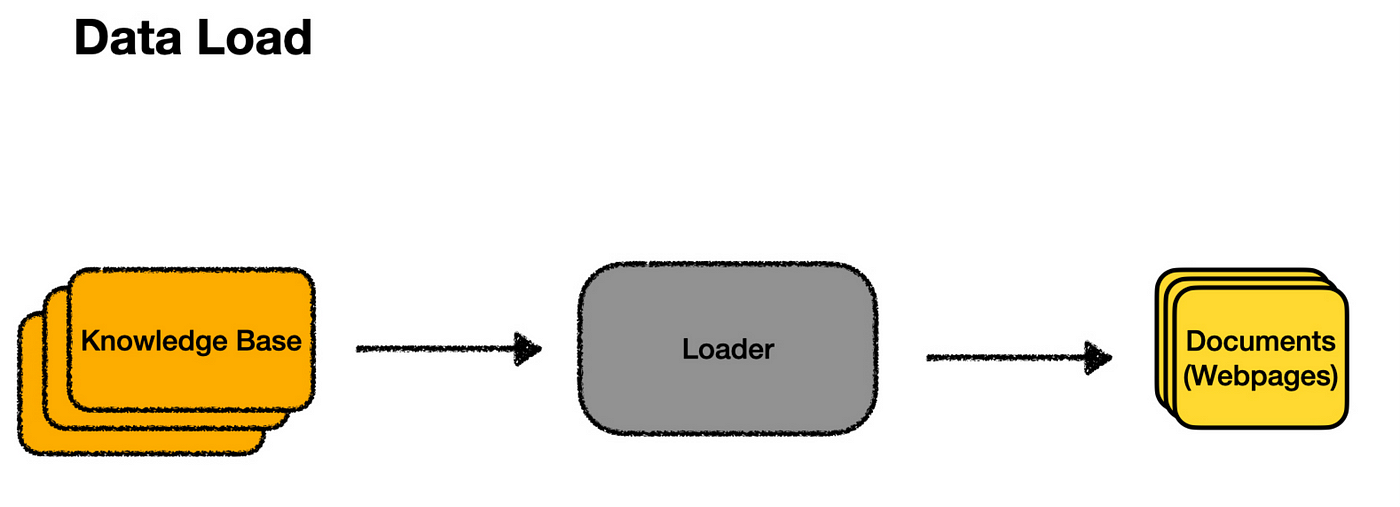
Once the loader has done its job, we’ll have a collection of documents corresponding to each page of the documentation site. Ideally, at this point, any extra markup has been removed, leaving just the structure and text.
Now, we can pass all these web pages to our embedding machine and use them as our knowledge snippets. However, each page might cover many topics, and the more content on a page, the less specific the embedding becomes. This can make our “closeness” search algorithm less effective.
The user’s question is more likely to match some specific piece of text within a page. This is where splitting comes in. By splitting, we break down each document into smaller, bite-sized, embeddable chunks better suited for search.
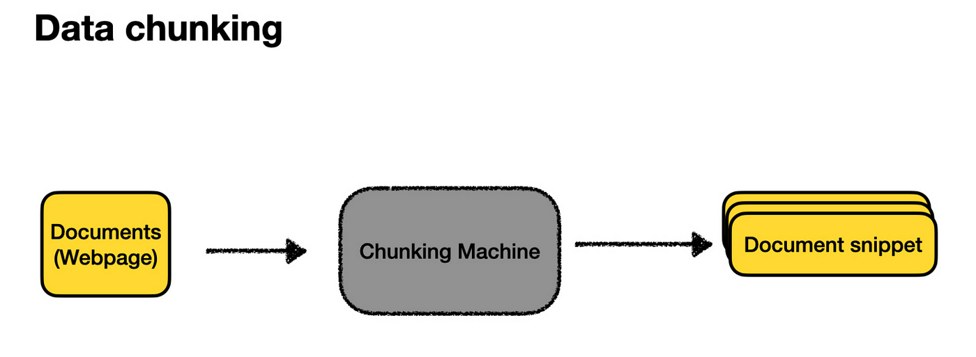
There’s an art to splitting your documents, including deciding how big the snippets should be (too big, and they don’t match queries well; too small, and they lack enough context to generate useful answers) and how to split them up (often by headings, if available). However, starting with a few sensible defaults is usually enough to get the ball rolling.
Once we’ve created these document snippets, we store them in our vector database, as described earlier, and voilà — we’re done!
Here’s the complete picture of indexing a knowledge base.
Recap of how it works:
What Types of Data Can be Stored in VectorDB?
Vector databases can handle different data types, such as text, images, audio, and more. Let’s understand how this works for different kinds of data:
1. Text Data
When it comes to text, embeddings are created to capture the meaning behind words, phrases, or even entire sentences. Techniques like Word2Vec, GloVe, or BERT are commonly used for this. These methods using semantic embeddings to better capture the relationship between words into vectors. Some popular approaches for text embeddings are:
Bag-of-Words (BoW) Model: This is a simple method for representing text by counting word occurrences. For example, if you have the sentence “I love cats,” this method might count the words and create a simple list like [1, 1, 1, 0], where each number represents a word from a list of possible words.
Word Embeddings (Word2Vec, GloVe): These techniques capture the context of words in a vector space. The word embedding method gives each word a more meaningful code based on how it’s used in sentences. So, “king” and “queen” might have similar codes because they’re related.
Pre-trained Language Models (BERT, GPT): Some advanced models, like BERT, generate more nuanced embeddings by understanding the context of words within sentences.
2. Image Data
For images, embeddings are usually created using convolutional neural networks (CNNs). Let’s say you have a photo of your pet dog and want to find dogs similar to him. The Vector DB could compare this photo to thousands of others and see pictures of similar dogs, even in different poses or locations.
These Convolutional Neural Networks are trained on large image datasets to recognize patterns, and the intermediate layers of the network can be used to create embeddings that represent the image’s content. It’s like turning a picture into a unique fingerprint. This fingerprint helps the Vector DB find other similar images. Standard methods for generating image embeddings are
Pre-trained Models: pre-trained models like ResNet, Inception, and MobileNet, which are trained on vast image datasets, can extract image features and create embeddings.
Autoencoders: Autoencoders compress and reconstruct images, with the compressed representation as the embedding.
3. Audio Data
Audio data can also be converted into embeddings using spectrogram analysis or deep learning models. The embeddings created for audio data capture the characteristics of the audio signal, making it possible to compare and search audio files.
Let’s say you are listening to a song and want to hear from the same genre. The Vector DB could find other similar songs based on the rhythm, melody, or instruments used. This is done by breaking the audio into patterns the database can understand and compare. Some methods for creating audio embeddings are:
Mel-Frequency Cepstral Coefficients (MFCCs): It is a feature extraction technique that captures the spectral shape of the audio signal.
Spectrogram-Based Embeddings: This technique of embeddings converts audio signals into visual spectrograms and then uses CNNs to create embeddings.
4. Multimodal Embeddings
Multimodal data consisting of different formats like text, images, and audio is handled by creating Multimodal embeddings stored in a shared space where similar items are close to each other, regardless of their original form. This enables cross-modal retrieval (finding related data across different formats) and classification.
Let’s say you have a caption that says “a red apple,” and you want to find the matching image. The Vector DB can understand the text and pictures and find the closest match. It’s like finding the right puzzle pieces from different boxes that fit together. Examples: OpenAI’s CLIP and BLIP models.
5. Other Data Types
For data types like tabular or time-series data, embeddings can be created using machine learning techniques such as autoencoders or clustering algorithms. For a spreadsheet with sales numbers, Vector DB might help one find patterns or predict future sales by comparing similar data from the past.
How is the Closest Match Found in a Vector DB?
Approximate Nearest Neighbour (ANN) algorithms are used to find the closest match for a query.
What is Approximate Nearest Neighbours (ANN)?
Let’s assume you’re in a vast library and trying to find books similar to the one you’re holding. Instead of checking every book, you could ask a librarian who knows the library well to show you a small section where similar books are likely to be. This is what ANN algorithms do. They help you find the “closest” matches without looking through everything.
These algorithms are called “approximate” because they focus on speed and efficiency, sometimes sacrificing a bit of accuracy to get results faster. But even with this trade-off, they still do an excellent job finding what you’re looking for.
How Does ANN Work?
ANN works by creating a map of all the data in the Vector DB. When you search for something, instead of comparing your query to every single piece of data, the algorithm quickly narrows down the options to a smaller group likely to be similar to your query called “candidate sets.” Then, it only compares your query to this smaller group, saving time and effort.
This approach is beneficial in areas like:
Recommendation systems: Finding products or content similar to what you’ve liked before.
Image retrieval: Locating pictures that look similar.
Natural language processing: Understanding and comparing the meanings of different texts.
Popular ANN Algorithms
There are several popular ANN algorithms, each unique way of finding the closest matches in a dataset. Here’s a simple, intuitive explanation of a few common ones:
1. Brute Force
Although not technically an ANN algorithm, as the name suggests, brute force is the most straightforward method and is a benchmark for comparing other algorithms. It’s like checking every item in a store to find the one that matches your list perfectly.
Brute force compares your query with every vector in the dataset to find the exact match. Because it checks everything, it guarantees to find the exact nearest neighbours. However, it’s not the fastest method, so it’s often used as a baseline to see how well other, more sophisticated algorithms perform.
2. Locality-Sensitive Hashing (LSH)
LSH is like a clever filing system that groups similar items. The idea is to hash or tag similar data points so that they end up in the same “bucket.” The dataset is hashed multiple times using different hashing functions to ensure that similar items collide and end up in the same bucket. When you search, the query is hashed the same way, and the algorithm checks the buckets where similar items are likely to be, making the search much faster than brute force.
3. K-D Trees
Think of K-D trees as a decision-making path that helps you find what you want. They are a type of binary search tree where data is split into two parts based on specific features (or dimensions) at each step. The algorithm keeps dividing the data until it has created a complete tree, where each branch represents a decision based on the data’s characteristics.
When you search for something, the algorithm follows the tree’s branches to find the closest match. While k-d trees are great for simple, low-dimensional data, they can struggle when dealing with more complex, high-dimensional data due to what’s known as the “curse of dimensionality,” where too many dimensions make the process less efficient.
4. Annoy (Approximate Nearest Neighbors Oh Yeah)
Annoy is like a forest of decision paths that quickly help you find similar items. Created by Spotify, this open-source library builds multiple binary search trees using random data splits. When you search, the algorithm checks multiple trees to find the nearest match.
One cool feature of Annoy is that it can use pre-made indexes stored in files, making it easy to share and load these indexes across different processes. Annoy is particularly good at handling complex, high-dimensional data. Spotify uses it to power its music recommendation engine, helping to match users with the songs they’ll love quickly.
5. Hierarchical Navigable Small World (HNSW) Graphs
HNSW is like a super-efficient network of roads connecting various points in an ample space. Each point in the network represents a piece of data, and the roads (or edges) link points are close to each other.
The network is built in layers; each layer gets more detailed as you move down. When searching for something, the algorithm starts at the top layer and works its way down, quickly zeroing in on the closest match.
HNSW is popular because it offers speed and accuracy, even in complex, high-dimensional spaces.
6. ScaNN (Scalable Nearest Neighbors)
ScaNN, developed by Google, is like a high-speed search engine designed to find similar items in massive, complex datasets. It uses a mix of techniques, including breaking down data into simpler parts (quantization), analyzing those parts separately (vector decomposition), and navigating through a network of related data points (graph-based search).
ScaNN is especially good at handling large-scale searches, making it fast and accurate.
7. Hybrid Approaches
Hybrid methods combine different algorithms to achieve the best of both worlds. By mixing various approaches, such as the ones mentioned above, hybrids aim to balance speed, accuracy, and efficiency.
References:
[1] https://scriv.ai/guides/retrieval-augmented-generation-overview/
[2] https://www.elastic.co/what-is/vector-database
[3] https://towardsdatascience.com/comprehensive-guide-to-approximate-nearest-neighbors-algorithms-8b94f057d6b6