
Search in the age of AI- Retrieval methods for Beginners
A deep dive into the workings of current Retrieval methods in Information Search for Absolute Beginners

The story of search and search engines is very intimately tied to language. Until recently, computers could not simulate human-level comprehension, finding information earlier was a tedious and error-prone process. The search engine earlier was much like when you use a library card catalog, matches the words you type with words in its catalog of information (its index). This is called lexical or keyword search. This process of locating information is iterative, manual, and often frustrating.
However, the landscape of search has been significantly transformed by the advent of OpenAI’s ChatGPT in 2022. ChatGPT powered by a large language model (LLM), generates text responses to text questions with remarkable accuracy. ChatGPT, along with other AI assistants, code generators, and agents, has dramatically altered people’s expectations about interacting with digital tools and sparked excitement around information retrieval in the digital sphere.
We are now on the cusp of a search revolution that merges the conversational abilities of chatbots and AI assistants with the rapid information processing capabilities of search engines. Techniques like retrieval-augmented generation (RAG) are being used to enhance the accuracy and relevance of search results.

This blog aims to acquaint readers with the emerging possibilities in the world of information retrieval, providing insights into semantic search and generative AI for builders, product managers, and executives. It will guide application developers on incorporating these technologies into applications, help product managers strategize their product integration, and assist executives in shaping their team’s direction towards harnessing the power of generative AI.
What is search and search Engine?
The purpose of search is to locate information that is relevant to a task at hand. Broadly speaking, whether you’re chatting with an AI chatbot or typing words into a search box, you are searching.
Search engines are programs that allow users to search and retrieve information from the vast amount of content available on the internet.
It produces a ranked list of texts (web pages, scientific papers, news articles, tweets, etc.) ordered by estimated relevance with respect to the user’s query
Search engines have two core capabilities — indexing and retrieval. To build a search experience, application builders send information to the engine as structured documents. Document, in this context, is a term of art referring to a single entity that the engine indexes and that search queries retrieve. The engine indexes the information in the fields of the search documents, providing fast matching and retrieval for text, numbers etc.
In modern search systems, machine learning and other strategies are employed to enhance the relevance of search results. These strategies include behavioural tracking, query rewriting, and personalization, which utilize user behavior signals such as clicks and purchases to improve the search experience.
Types of search:
Two types of searches are possible and in practise in Information Retrieval(IR) and they are Lexical search and Semantic search. Let’s explore how each one of these searches works.
Lexical Search:
Lexical search is the most basic form of searching, operating directly with language.
What is lexical search?
It breaks down large chunks of unstructured text into individual words, matching these words with the text in a query.
Let’s take an example of a pet bird recommendation website. The creators of this site use pet descriptions as the body of documents for their search engine. Two such text blocks describing Cocktails and African Greys are shown below:
Text sample A : Cockatiels are among the most communicative and emotional birds. they are much more well known for their quirk of mimicking sounds around them including phones, alarms, and even outdoor birds. These smart little birds crave social interaction and require an owner who can provide them with the time and attention they need in order to thrive and prevent loneliness, or depression.
Text sample B: African grey parrots are believed to be the smartest birds in the world and are capable of learning a huge vocabulary. Because of their outsized intelligence, these parrots need somewhere in the vicinity of 5 hours of stimulation every day to keep from falling into boredom or depression. Those looking to make a serious commitment to a forever friend can find an intelligent and loving companion in an African grey parrot.
When searching for singing birds, text sample A appears to be a more suitable match than text sample B.
The problem of search is typically addressed by most search engines in three stages — matching, merging, and ranking. Let’s explore and understand how each of these stages work.
Matching:
The process of normalizing text for matching is typically done at index time, when a document is added to the index, and at query time, when the user runs a search. In a search engine using lexical search, the process of normalizing text for matching involves several steps.
Segmentation - During segmentation, the search engine eliminates punctuation and converts terms to lowercase. This ensures that Run matches with run.
Stemming - Language-specific stemming rules remove common inflections. Consequently, Run would match with run, runs, and running.
Stop-word Filtering - A stop-word filter eliminates common terms such as articles (a, an, the, etc.) that have low value for matching due to their prevalence in almost every document.
Synonym Matching — Finally, synonyms are added to match terms across common groupings. For instance, happy and joyful might be used as synonyms for glad.
This discussion primarily centers on the English language analyzer. The topic of searching across multiple languages is extensive, encompassing aspects such as index design, language analysis, and tenancy of index, cluster, and document.
The preprocessed text samples look like this:
Text sample A (cocktails): cockatiel among commun emot bird
much well known quirk mimick sound around includ phone alarm
even outdoor birdsthes smart littl bird crave social interact
requir owner provid time attent need order thrive prevent
loneli depress recommend keep cockatiel pair get lone leav

Text sample B (African Grey): african grey parrot believ
smartest bird world capabl learn huge vocabularybecaus outsiz
intellig parrot need somewher vicin 5 hour stimul everi day
keep fall boredom depress look make seriou commit forev friend
find intellig love companion african grey parrot
The output looks odd. What’s going on here? You can see that stop words are removed. We haven’t applied synonyms, so there are no additional terms. Stemmer has transformed the text by stemming.For example, communicative becomes commun, and emotional becomes emot.
Of course, textual queries undergo a similar analysis. The query “playing and singing bird” is rendered as ”play sing bird”
To match a query, search engines use an inverted index. An index in a book maps words to the numbers of pages where those words occur; to find something, you go to the index, look up a term, and go to the page number(s) indicated until you find what you are looking for. Similarly, an inverted index in a search engine maps terms onto the document IDs for documents that contain those terms. The search engine looks up the terms in the index, then combines the sets of document IDs to determine the match.
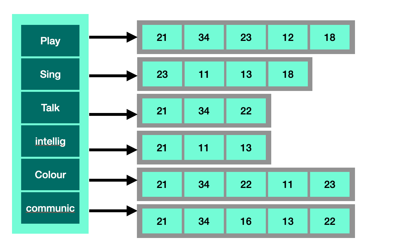
The above diagram shows some of the terms that might be in our example corpus. On the left, you see the terms index; on the right are the posting lists or document index for each entry. During matching, the engine looks up the term in the terms index. To match ”play sing bird”, it looks up the analyzed terms—play, sing, and bird—to get the posting lists [21,34,23,12,18, 43] and [23, 11, 13, 18]
Merging
The second phase of search is merging the posting lists to get a single set of matches. Search engines use set math to compute the match. If the application wants to match all terms in the query, it will use an AND operator for the query, and the engine will compute the intersection of the posting lists—in this case, [23,11], or an empty set. In most cases, the application will use an OR operator—a union—to retrieve [21,34,23,12,18, 43,23, 11, 13, 18]. It relies on scoring and sorting to bring the most relevant documents to the top.
Reranking
In the last step of the search process, called ranking, search engines use a special algorithm to determine the relevance of a document to a specific search query. This algorithm, known as Term Frequency-Inverse Document Frequency (TF-IDF), operates on the overall statistics of the text. Here’s how it works:
Rare terms or words in the document receive high scores.
Common terms or words, on the other hand, receive low scores.
The score of a document for a particular search query is calculated by adding up the scores of the terms that match the query. This total is then multiplied by the number of times these terms appear in the document.
During the ranking phase, the search engine arranges all the documents that match the search query based on their scores. The documents with the highest scores are placed at the top of the search results, while those with lower scores appear further down the list. This process ensures that the most relevant documents are presented to the user first, making it easier for them to find the information they’re looking for.
In simpler terms, let’s say that you’re looking for a recipe for chocolate chip cookies. The search engine will first find all the web pages that mention chocolate chip cookies. Then, it will rank these pages based on how often the terms “chocolate chip cookies” appear and how important these terms are in the context of the page. The most relevant and useful pages will be shown to you at the top of the search results.
Implementation of Lexical search
Let’s see how to do a simple Lexical search in practice using nltk package in python.
import nltk
nltk.download('punkt')
nltk.download('stopwords')
from nltk.corpus import stopwords
from nltk.tokenize import word_tokenize
import re
from sklearn.feature_extraction.text import TfidfVectorizer
# Sample corpus of documents
corpus = ['Cockatiels are among the most communicative and emotional birds. they are much more well known for their quirk of mimicking sounds around them including phones, alarms, and even outdoor birds.these smart little birds crave social interaction and require an owner who can provide them with the time and attention they need in order to thrive and prevent loneliness, or depression. It’s recommended to keep cockatiels in pairs so they do not get lonely when you have to leave the home; single cockatiels can be kept as pets, but they require near-constant attention from their owner to stay in high spirits.',
          'African grey parrots are believed to be the smartest birds in the world and are capable of learning a huge vocabulary.Because of their outsized intelligence, these parrots need somewhere in the vicinity of 5 hours of stimulation every day to keep from falling into boredom or depression. Those looking to make a serious commitment to a forever friend can find an intelligent and loving companion in an African grey parrot.'
         ]
# Define a function to preprocess the text
def preprocess_text(text):
    # Convert to lower case
    text = text.lower()

    # Remove punctuation
    text = re.sub(r'[^\\w\\s]', '', text)

    # Tokenize the text
    tokens = word_tokenize(text)

    # Remove stopwords
    tokens = [token for token in tokens if token not in stopwords.words('english')]

    # Perform stemming
    stemmer = nltk.stem.PorterStemmer()
    tokens = [stemmer.stem(token) for token in tokens]

    # Perform lemmatization
    lemmatizer = nltk.stem.WordNetLemmatizer()
    tokens = [lemmatizer.lemmatize(token) for token in tokens]

    # Join the tokens back into a string
    text = ' '.join(tokens)

    return text

# Preprocess the corpus
corpus = [preprocess_text(doc) for doc in corpus]
print('Corpus: \\n{}'.format(corpus))
# Create a TfidfVectorizer object and fit it to the preprocessed corpus
vectorizer = TfidfVectorizer()
vectorizer.fit(corpus)
# Transform the preprocessed corpus into a TF-IDF matrix
tf_idf_matrix = vectorizer.transform(corpus)
# Get list of feature names that correspond to the columns in the TF-IDF matrix
print("Feature Names:\\n", vectorizer.get_feature_names_out())
# Print the resulting matrix
print("TF-IDF Matrix:\\n",tf_idf_matrix.toarray())Semantic search
Step 1. Import Necessary Libraries
nltk(Natural Language Toolkit) is used for text preprocessing tasks like tokenization, stopword removal, stemming, and lemmatization.sklearn.feature_extraction.text.TfidfVectorizeris used to compute the TF-IDF matrix for the processed corpus, a crucial step in representing the importance of terms in documents.
2. Downloading NLTK Resources
nltk.download('punkt')
nltk.download('stopwords')
These commands download essential NLTK components:
'punkt'for tokenizing sentences into words.'stopwords'for removing common words like "and," "the," etc.
3. Sample Corpus
The corpus contains two sample documents (descriptions of bird’s characteristics), which will be processed further.
4. Text Preprocessing Function
The preprocess_text(text) function carries out a series of text cleaning and transformation steps:
a. Convert to Lowercase:- This ensures uniformity by converting all text to lowercase.
text = text.lower()b. Remove Punctuation: This regular expression removes any characters that are not alphanumeric or whitespace, effectively stripping punctuation.
text = re.sub(r'[^\\w\\s]', '', text)c. Tokenization: The text is split into individual words (tokens) using word_tokenize().
tokens = word_tokenize(text)d. Stopword Removal: Common stopwords are removed from the token list to reduce noise in the data.
tokens = [token for token in tokens if token not in stopwords.words('english')]e. Stemming: Stemming reduces words to their root forms using the Porter Stemmer. For example, “playing” becomes “play.”
stemmer = nltk.stem.PorterStemmer()
tokens = [stemmer.stem(token) for token in tokens]
f. Lemmatization: Lemmatization further reduces words to their base form, accounting for the context. For example, “better” might lemmatize to “good.”
lemmatizer = nltk.stem.WordNetLemmatizer()
tokens = [lemmatizer.lemmatize(token) for token in tokens]
g. Rejoin Tokens: The tokens are joined back into a string, now cleaner and more concise.
text = ' '.join(tokens)5. Apply Preprocessing: This processes each document in the corpus using the preprocess_text function, preparing them for TF-IDF transformation.
corpus = [preprocess_text(doc) for doc in corpus]6. TF-IDF Vectorization
vectorizer = TfidfVectorizer()
vectorizer.fit(corpus)TfidfVectorizer()is initialized to convert the corpus into a matrix of TF-IDF features.vectorizer.fit(corpus)computes the term-document matrix based on the preprocessed text.
7. Transform the Corpus
tf_idf_matrix = vectorizer.transform(corpus)This step converts the processed corpus into a sparse matrix representation of TF-IDF values, where each row corresponds to a document, and each column corresponds to a term.
8. Extract and Display Features and TF-IDF Matrix: Next let us print the feature names (terms) extracted from the corpus. The matrix is converted into a 2D array, displaying the TF-IDF weights for each term in each document. These weights reflect the importance of terms in the context of the corpus
print("Feature Names:\\n", vectorizer.get_feature_names_out())
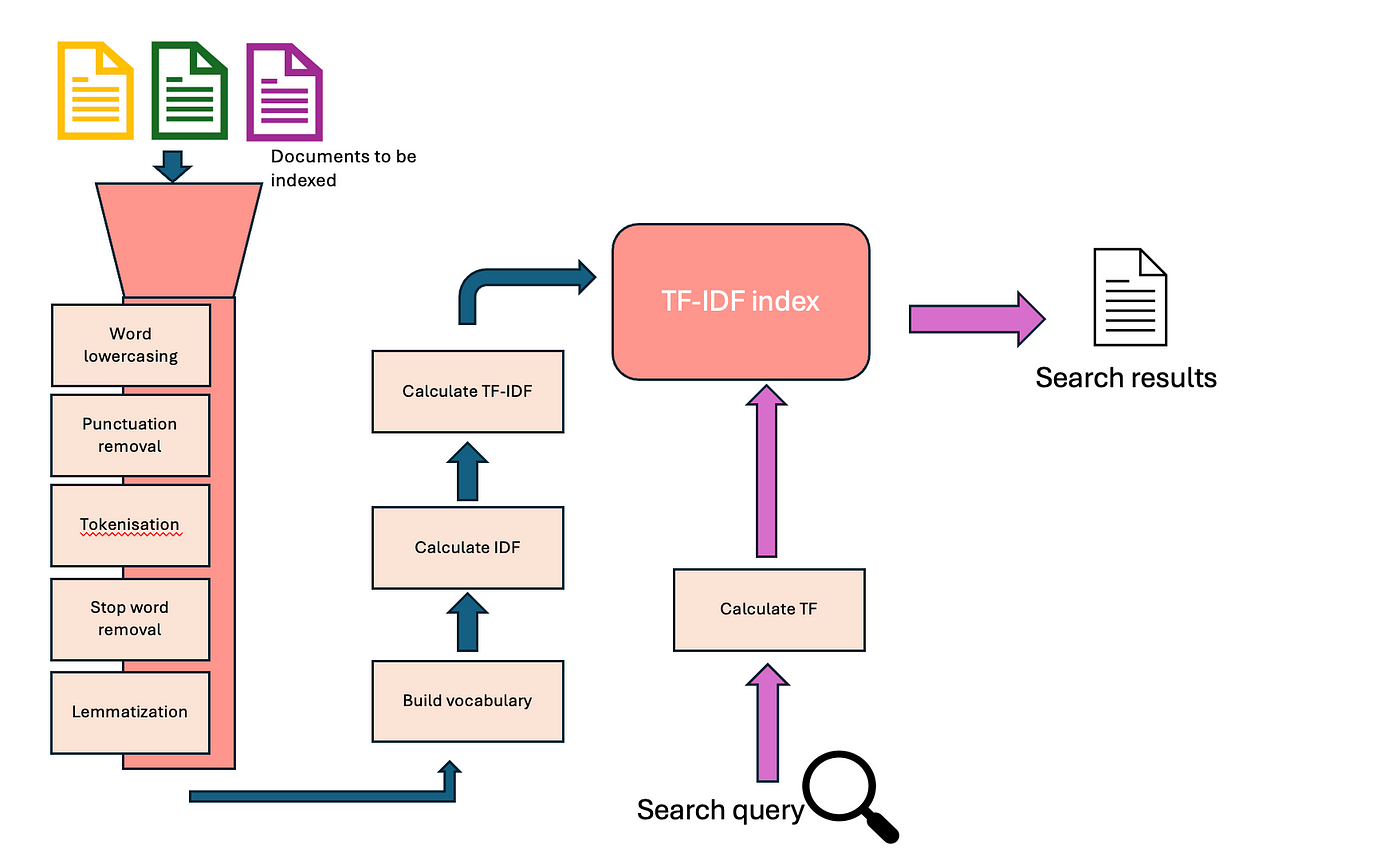
print("TF-IDF Matrix:\\n",tf_idf_matrix.toarray())The flow diagram below should summarise the workings of lexical search methods like TF-IDF or BM25
2. Semantic Search:
Semantic search is a method used by computers and machine learning (ML) models to understand and process natural language.
What is semantic search?
The basic idea behind semantic search is using vectors to represent the meaning of words in a way that allows for meaningful comparisons and combinations.
By training ML models on large datasets, we can create vectors that capture the subtle nuances of language, enabling more accurate and intuitive search results. These models only comprehend numbers, so to work with language, they need to convert it into numerical form. This is where ‘vectors’ come into play.
Vectors and embeddings
Vectors, also known as ‘embeddings’ in semantic search, are a way of representing natural language as a set of values across multiple dimensions. The goal of training ML models for search engines is to create a model that generates vectors that are close together for text with similar meanings and far apart for text with different meanings.
Picture a 512-dimension vector, which means it has 512 values along various axes. However, visualizing 512 dimensions is not something we can easily do!
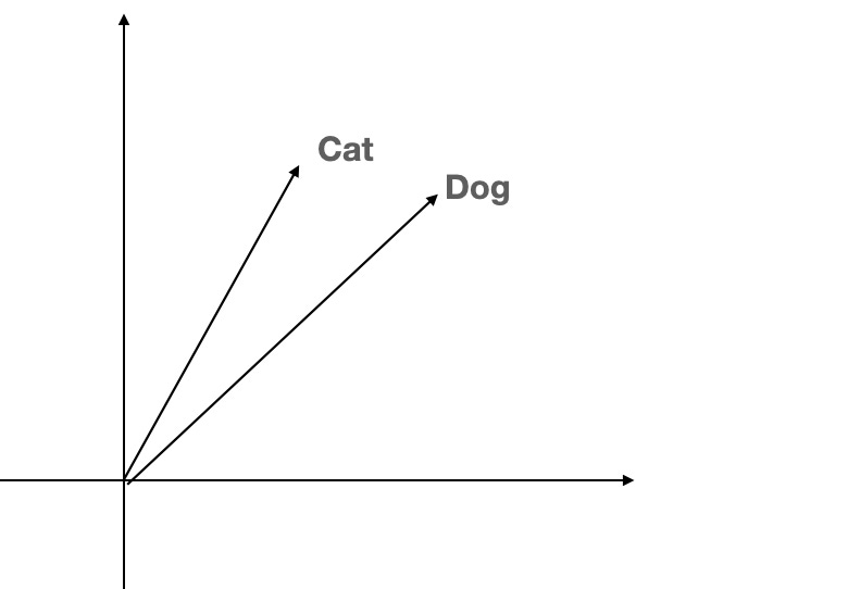
Let’s make it simpler. Think of assigning a unique number to each animal: ‘cat’ = 1, ‘dog’ = 2, ‘elephant’ = 3, and so on. But it doesn’t make sense to say ‘cat’ + ‘dog’ = ‘elephant’.
To improve this, we expand to two numbers, similar to plotting points on a map:
cat = (1,0)
dog = (0,1)
elephant = (0,2)
tiger = (1,2)
But there’s still a problem. Adding ‘cat’ and ‘elephant’ gives (1,2), which equals ‘tiger’. Clearly, adding more dimensions is necessary — but how many do we need?
Dimensionality: Sparse retrieval and dense retrieval
One solution is to use as many dimensions as there are words in the vocabulary. This is often called ‘sparse’, ‘keyword’, or ‘one-hot encoding’. However, sparse vectors can’t combine in a meaningful way. For instance, adding ‘animal’ and ‘pet’ shouldn’t result in ‘elephant’ or ‘lion’. But it would make sense if it equaled ‘dog’ since a dog is also a common pet.
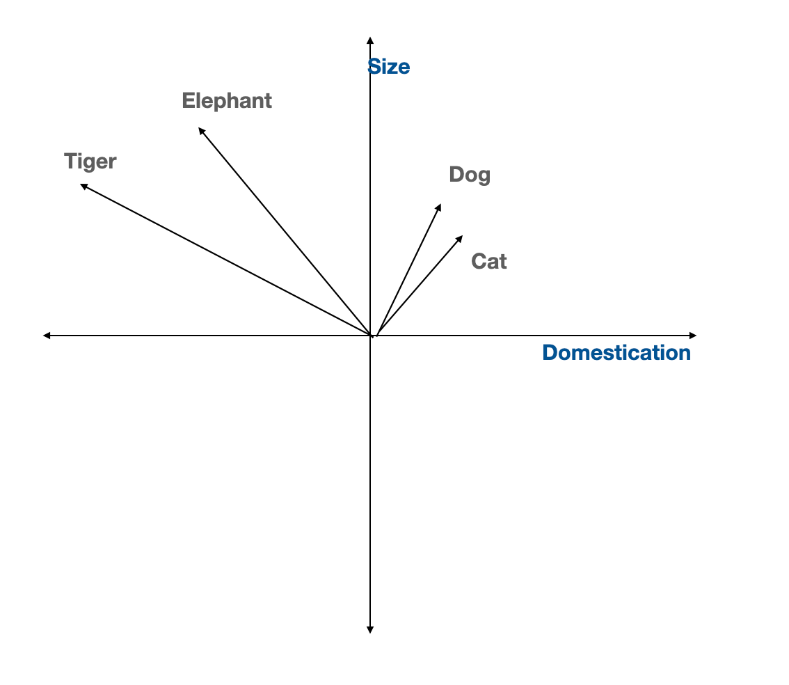
To better capture this kind of natural understanding, we use vectors with fewer dimensions than the total number of animals. These are called ‘dense vectors’, commonly used in modern machine learning models. For example, imagine a two-dimensional space where one axis represents ‘size’ and the other represents ‘domestication’. In this space, the vector for ‘domestic animal’ might be close to the vector for ‘dog’, while the vector for ‘wild animal’ might be farther away, near ‘lion’.
what is semantic search?
The core concept of semantic search is using vectors to represent the meaning of words in a way that allows for meaningful comparisons and combinations.
By training ML models on large datasets, we can create vectors that capture the nuances of language, enabling more accurate and intuitive search results.
Semantic search Process Flow:
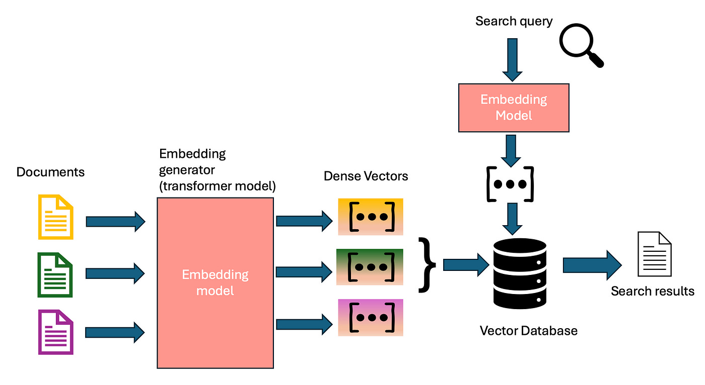
In semantic search, the search application uses an LLM to create a vector for each document in the corpus. When a user runs a search, the application encodes the text of that search query with the same LLM to produce a vector in the same space. It then uses a distance function to produce a score for the query/document pairs and ranks the results by that score.
BERT models for encoding meanings into vectors
BERT models can be used for encoding meaning to vectors? but why BERT? why not any other variants of transformer models, or deep learning models?
We know transformer architecture typically has two components, an encoder and a decoder. BERT, however, only uses the encoder component of the transformer. BERT is just several repeated layers with (bidirectional, multi-headed) self-attention and feed-forward transformations, each followed by layer normalization and a residual connection.
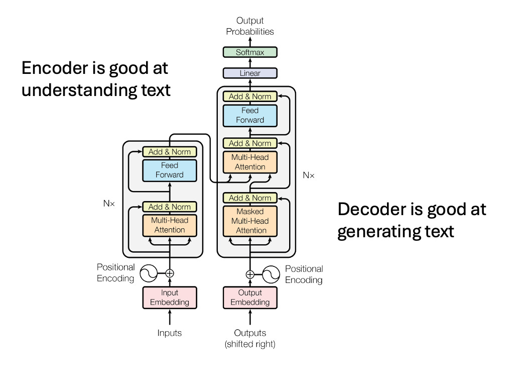
Encoder component of transformer is very good at understanding the natural language and that’s essentially why BERT models are good at understanding and representing language. There are two types of BERT models in particular that we use for searching and retrieval purpose — bi-encoders and cross-encoders.
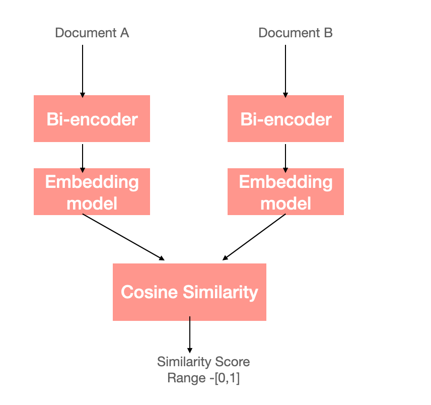
Bi-encoders are one of the basic dense retrieval algorithms used in the field. Bi-encoders take a sequence of text as input and produce a dense vector as output. The vectors produced by bi-encoders are semantically meaningful — similar sequences of text produce vectors that are nearby in the vector space. When you run a search, it matches your query’s vector to documents with the closest vectors, often using algorithms like cosine similarity. This makes finding the most relevant content quicker and more efficient.
Algorithms like hierarchical navigable small word (HNSW), we be used to make this process even faster. HNSW helps perform “approximate nearest neighbor” searches, so instead of searching everything, it narrows down the search to a smaller group likely to be similar to your query called “candidate sets”. Like what we did in lexical search, we can store document vectors within a database like Elastic or OpenSearch and build an HNSW search index. Then, a bi-encoder can be used to produce a vector for the user’s query and then we can perform a vector search to find the most similar documents using appropriate distance metrics.
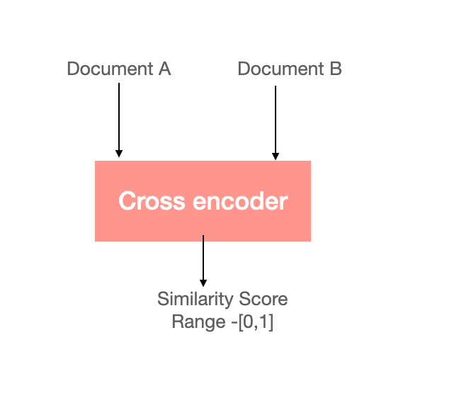
Cross-encoders take a different approach. Instead of creating separate vectors for the query and document, they process both together. See the diagram below to understand cross-encoders more. This allows them to make a much more accurate similarity score. The downside? It is computationally expensive, which means it’s not always practical for large-scale searches.
Both bi-encoders and cross-encoders are often built using the BERT model, which is a transformer-based architecture. Understanding BERT’s structure and how it works under the hood is essential for improving search systems. While cross-encoders are precise, bi-encoders strike a balance between speed and accuracy, making them a go-to choice for most vector-based search systems today.
How BERT Prepares Text for Understanding?
The first step in understanding how BERT, or any encoder-only model, works is by getting to know how it processes its input. While it might seem simple — just feed in a sentence, right? — there’s a bit more going on behind the scenes. Before BERT can understand text, it has to break it down into a form it can digest. This is where tokenization comes in.
Think of tokenization as cutting a sentence into small, manageable pieces called tokens. These tokens could be entire words or even parts of words. Tools like BPE (Byte Pair Encoding) or SentencePiece help with this. They split the text into tokens, transforming the input into something BERT can work with.
But there’s more to it. BERT also relies on a few special tokens to help it navigate through the text:
[CLS]: This token is placed at the very beginning of the text. It’s like BERT’s personal note-taking tool—it captures the overall meaning of the entire sequence.[SEP]: When multiple sentences are involved, the[SEP]token acts as a boundary, separating one sentence from the next. This helps BERT differentiate between different chunks of text.[EOS]: At the end of the sequence, the[EOS]token signals that the text has finished. It’s like putting a period at the end of a paragraph, making sure BERT knows where the text ends.
These tokens play a critical role in helping BERT understand not just individual words but also the relationships between them, making its text representations more meaningful.
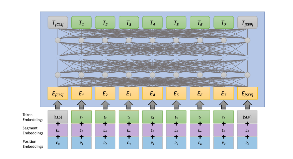
Embedding the Tokens: How BERT Understands Position?
Once the input text has been tokenized, each token needs to be embedded — that is, converted into a numeric vector that the model can understand. To do this, BERT uses a large embedding layer, which acts like a lookup table, transforming each token into a unique vector. But before these vectors get processed by the model, something important happens and that is positional embedding.
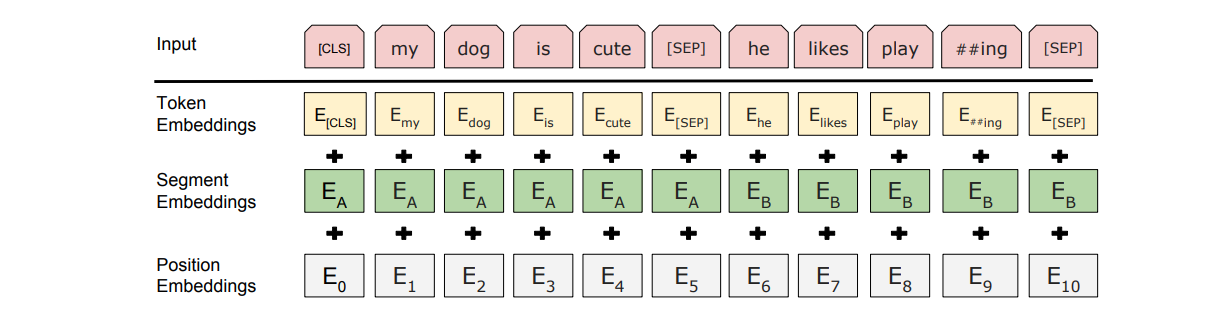
Why does position matter? Well, language has structure, and the order of words is crucial for meaning. To help BERT understand the placement of each token, a positional embedding is added to the token vectors. This positional information helps BERT recognize where each word fits within the sentence, allowing it to capture more than just the meaning of individual words — it also understands how the words relate to each other.
Bidirectional Self-Attention: Seeing the Whole Picture
Self-attention is the secret sauce behind BERT’s ability to process language so effectively. Although a deep dive into self-attention is outside the scope of this post, the gist is this: self-attention allows BERT to transform each token by looking at all other tokens in the sequence. But here’s the key — BERT uses bidirectional self-attention, meaning it doesn’t just look at the words that came before the token; it also considers the words that come after it.
Imagine reading a sentence one word at a time versus having the whole sentence in front of you. Bidirectional self-attention gives BERT that full-sentence perspective, allowing each word to be understood in the context of the entire sequence.
Feed-Forward Transformation: Enhancing Each Token
Next comes the feed-forward transformation, which serves a different purpose. Unlike self-attention, which looks at how tokens interact with each other, feed-forward transformations focus on individual tokens. Every token in the sequence goes through the same transformation: a couple of linear operations with a ReLU activation function in between. Think of this as polishing each token’s representation, one at a time. After this, normalization is applied to ensure the outputs are balanced and ready for the next step.
Putting It All Together: How BERT Learns?
Both the bidirectional self-attention and feed-forward transformations work in tandem, each contributing something unique. Self-attention helps the model understand the bigger picture by considering how all tokens relate to one another, while the feed-forward transformation fine-tunes each token’s individual representation. Together, these processes allow BERT to capture complex patterns and relationships in text, giving it the ability to excel in tasks like search, question-answering, and text classification.
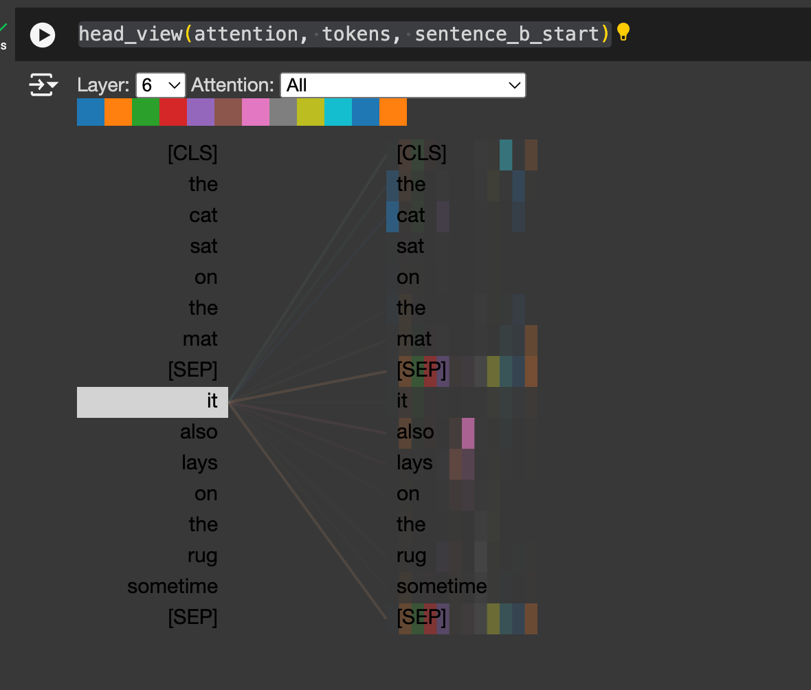
To better understand how attention works, I suggest that you read this blog by Jay. Now, let’s try to visualize how attention works in transformers using bertviz python package. BertViz is an interactive tool for visualizing attention in Transformer language models such as BERT, GPT2, or T5. It can be run inside a Jupyter or Colab notebook through a simple Python API
# Load model and retrieve attention weights
from bertviz import head_view, model_view
from transformers import BertTokenizer, BertModel
model_version = 'bert-base-uncased'
model = BertModel.from_pretrained(model_version, output_attentions=True)
tokenizer = BertTokenizer.from_pretrained(model_version)
sentence_a = "The cat sat on the mat"
sentence_b = "It also lays on the rug sometime"
inputs = tokenizer.encode_plus(sentence_a, sentence_b, return_tensors='pt')
input_ids = inputs['input_ids']
token_type_ids = inputs['token_type_ids']
attention = model(input_ids, token_type_ids=token_type_ids)[-1]
sentence_b_start = token_type_ids[0].tolist().index(1)
input_id_list = input_ids[0].tolist() # Batch index 0
tokens = tokenizer.convert_ids_to_tokens(input_id_list)
### The head view visualizes attention in one or more heads from a single Transformer layer.
head_view(attention, tokens, sentence_b_start)
Visualizing the attention of Sentence A — “The cat sat on the mat” and Sentence B- “It also lays on the rug sometime” shows how layer 6 is able understand how word ‘it’ refers to ‘cat’.
I think by now, you could have understood basic workings of BERT models. Having said vanilla BERT models work poorly for semantic similarity and clustering tasks, you might wonder: How can we adapt these models to produce more useful embeddings for semantic search? Adapting BERT models in this way is not very difficult. We just need to finetune these models using a siamese or triplet network structure to derive semantically meaningful text or document representations -sBERT models or Sentence-BERT: Sentence Embeddings using Siamese BERT-Networks. sBERT models are implemented in a Python library, called Sentence Transformers, that is built on top of the PyTorch and HuggingFace. This package openly provides tons of state-of-the-art models — including both bi-encoders and cross-encoders — and makes it easy to use these models and efficiently finetune them on your own data. Because this package is based upon sBERT, SentenceTransformer embeddings are semantically meaningful — similar sentences yield embeddings that are close in vector space.
Example of semantic search using SentenceTransformer:
"""This is a simple application for sentence embeddings: semantic searchWe have a corpus with various sentences. Then, for a given query sentence,we want to find the most similar sentence in this corpus.This script outputs for various queries the top 5 most similar sentences in the corpus."""
import torch from sentence_transformers
import SentenceTransformer
embedder = SentenceTransformer("all-MiniLM-L6-v2")
# Corpus with example sentencescorpus = [
    "A man is eating food.",
    "A man is eating a piece of bread.",
    "The girl is carrying a baby.",
    "A man is riding a horse.",
    "A woman is playing violin.",
    "Two men pushed carts through the woods.",
    "A man is riding a white horse on an enclosed ground.",
    "A monkey is playing drums.",
    "A cheetah is running behind its prey.",
]
# Use "convert_to_tensor=True" to keep the tensors on GPU (if available)corpus_embeddings = embedder.encode(corpus, convert_to_tensor=True)
# Query sentences:queries = [
    "A man is eating pasta.",
    "Someone in a gorilla costume is playing a set of drums.",
    "A cheetah chases prey on across a field.",
]
# Find the closest 5 sentences of the corpus for each query sentence based on cosine similaritytop_k = min(5, len(corpus))
for queryin queries:
    query_embedding = embedder.encode(query, convert_to_tensor=True)
# We use cosine-similarity and torch.topk to find the highest 5 scoressimilarity_scores = embedder.similarity(query_embedding, corpus_embeddings)[0]
    scores, indices = torch.topk(similarity_scores, k=top_k)
    print("\\nQuery:", query)
    print("Top 5 most similar sentences in corpus:")
for score, idxin zip(scores, indices):
        print(corpus[idx], "(Score:{:.4f})".format(score))
I hope you enjoyed reading this in-depth blog on search or Information Retrieval. Please do follow me for more such content on AI and ML.
References:
[1] Devlin, Jacob, et al. “Bert: Pre-training of deep bidirectional transformers for language understanding.” arXiv preprint arXiv:1810.04805 (2018).
[2] Reimers, Nils, and Iryna Gurevych. “Sentence-bert: Sentence embeddings using siamese bert-networks.” arXiv preprint arXiv:1908.10084 (2019).
[3] Jimmy Lin, Rodrigo Nogueira, and Andrew Yates. “Pretrained Transformers for Text Ranking: BERT and Beyond” https://arxiv.org/pdf/2010.06467