
Lesson 5.1: What Is a Vector Database and How Is It Different from a Regular Database?

You’ve learned how embeddings transform text into meaningful vectors, but where do those vectors actually live, and how do you search through millions of them in milliseconds? In this lesson, we confront a question every developer asks: “Why can’t my trusty PostgreSQL handle this?” The answer reveals why vector databases exist as an entirely new category of infrastructure, built around a fundamentally different question than anything your B-tree index was designed to answer.
The Developer’s Question:
You’ve been writing database queries your entire career. They all look something like this:
Example:
SELECT * FROM customers WHERE email = ‘alice@example.com’;
SELECT * FROM orders WHERE status = ‘shipped’ AND date > ‘2024-01-01’;
SELECT * FROM products WHERE category = ‘electronics’ AND price < 500;
Every single one of these queries asks the same fundamental question:
“Find me rows where this column exactly matches (or falls within) this value.”
Your database is really good at this. It uses indexes, scans sorted structures, and returns precise results. Either a row matches or it doesn’t. There’s no “kind of matches” or “close enough.” It’s binary, yes or no.
Now, here’s the question that RAG applications ask:
“Find me the documents whose meaning is most similar to what this user just asked.”
There’s no column to match on. No exact value to compare. You’re not looking for equality. You’re looking for closeness in meaning, which, as we learned in Module 4, has been translated into closeness in a high-dimensional vector space.
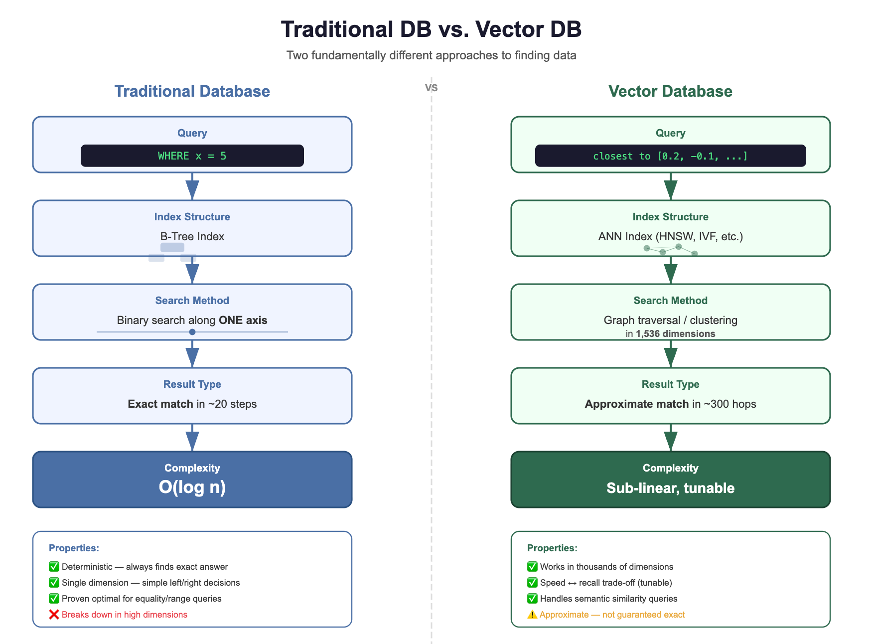
This is a fundamentally different operation:
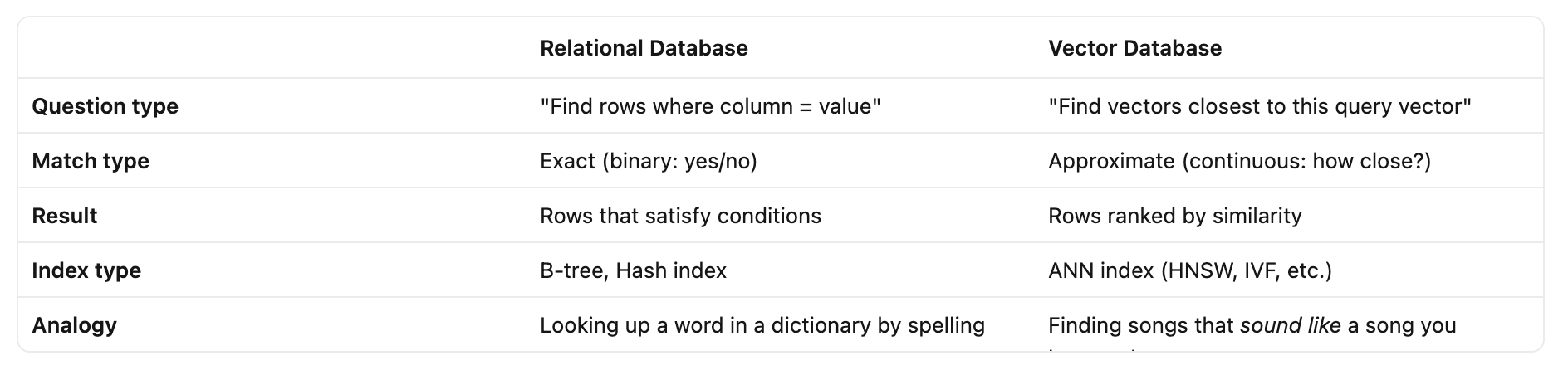
Both are useful. But they solve completely different problems. And they require completely different internal machinery.
Why Your Trusty B-Tree Index Can’t Help Here?
Okay, so you need to find close vectors instead of exact matches. But you’re a pragmatic developer. Your first instinct is:
“Can’t I just store vectors in PostgreSQL and write a query with some distance function? Maybe add an index?”
Let’s walk through why this breaks down, step by step.
How B-Trees Work?
A B-tree is the workhorse index behind almost every relational database. Here’s its core trick:
It sorts your data along a single dimension.
Imagine you have a million customer IDs. A B-tree organizes them like a phone book, sorted, with hierarchical tabs that let you jump to the right section quickly.
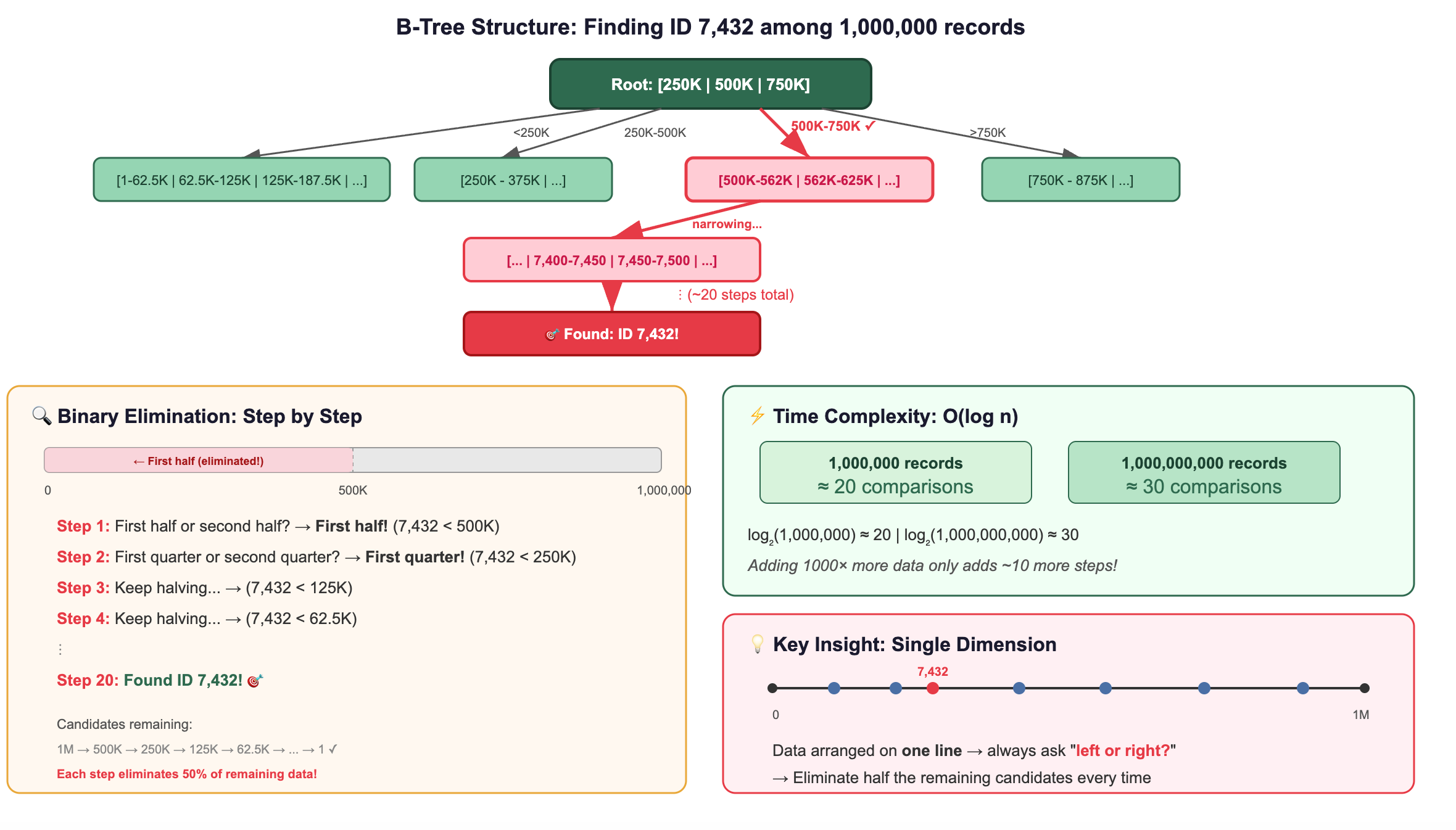
This works because data is arranged along one line, a single dimension. You can always ask “left or right?” and eliminate half the remaining candidates.
What Happens When You Add Dimensions?
Now let’s see what happens as we increase dimensions:
1 Dimension (a number line):

A B-tree handles this beautifully. Sort the numbers, binary search, done. You can immediately eliminate everything below 20 and above 40.
2 Dimensions (a flat plane):
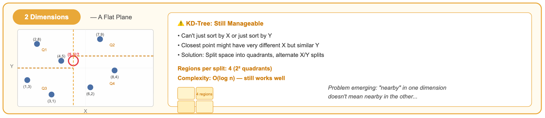
With 2D, you can divide space into 4 quadrants. A KD-tree alternates splitting by X and Y. It works reasonably well.
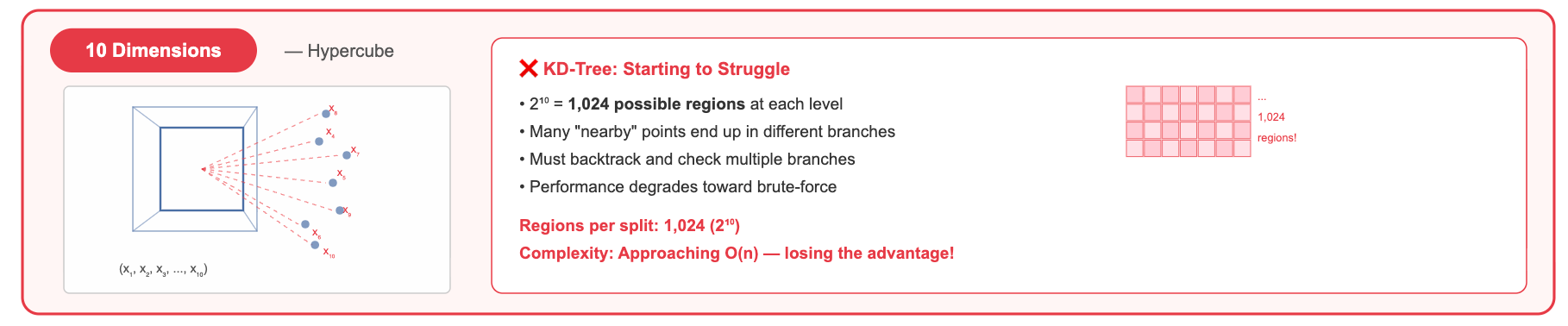
10 Dimensions:
Now you have 2¹⁰ = 1,024 possible quadrants (orthants). A tree split eliminates a smaller and smaller fraction of the data with each decision. You start needing to explore many branches.
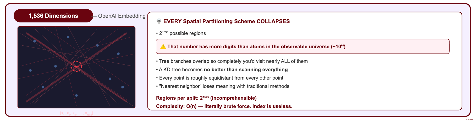
1,536 Dimensions (a typical OpenAI embedding):
You'd have 2¹⁵³⁶ possible orthants, ca number so large it dwarfs the number of atoms in the observable universe (≈2²⁶⁶). No tree structure can meaningfully partition this space with a reasonable number of splits.
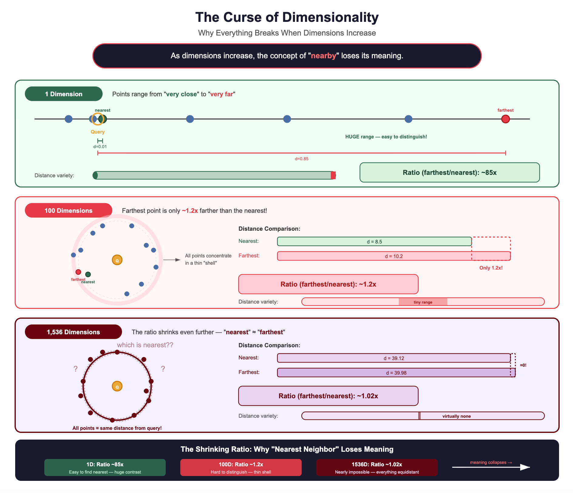
The Curse of Dimensionality: Why Everything Breaks when dimensions increases?
This phenomenon has a name: the curse of dimensionality. Here’s what it means intuitively:
As dimensions increase, the concept of “nearby” loses its meaning.
In high-dimensional space, a strange thing happens: all points become roughly equidistant from each other.
Why does this happen? Consider two random vectors in 1,536 dimensions. Each dimension contributes a small random amount to the total distance. By the law of large numbers, when you sum 1,536 small random contributions, the total concentrates around its expected value. Every pair of random vectors ends up with nearly the same total distance.
It’s like flipping 1,536 coins: while any single coin is random, the total number of heads will almost always be close to 768. Similarly, the distance between any two random high-dimensional vectors will almost always be close to the same value.
When all distances look similar, a tree-based index can’t make meaningful “left or right” decisions. Every branch looks equally promising. You end up checking almost everything anyway.
This is why you cannot use a B-tree (or any traditional index) for high-dimensional vector search.
The Breakthrough: Approximate Nearest Neighbor (ANN)
The core idea that makes vector databases possible is ANN, which builds on the principle.
You don’t need the exact nearest vectors. You need vectors that are close enough, found fast enough.
This is called Approximate Nearest Neighbor (ANN) search. And it changes the game entirely.
Why “Approximate” is a Brilliant Approach?
Let’s make this concrete with a RAG scenario.
A user asks: “How do I configure SSL certificates in our Kubernetes cluster?”
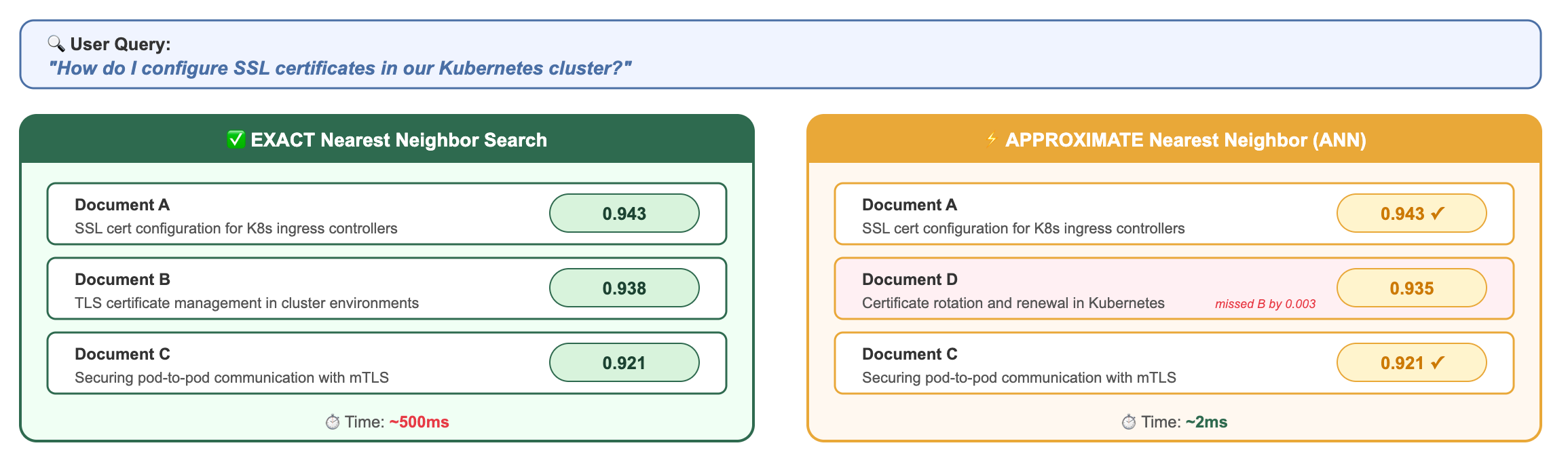
Does the user care that they got Document D (score 0.935) instead of Document B (score 0.938)?
Absolutely not. Both documents are highly relevant. Both will help the LLM generate a correct answer. The difference is imperceptible in the final output.
But the performance difference?
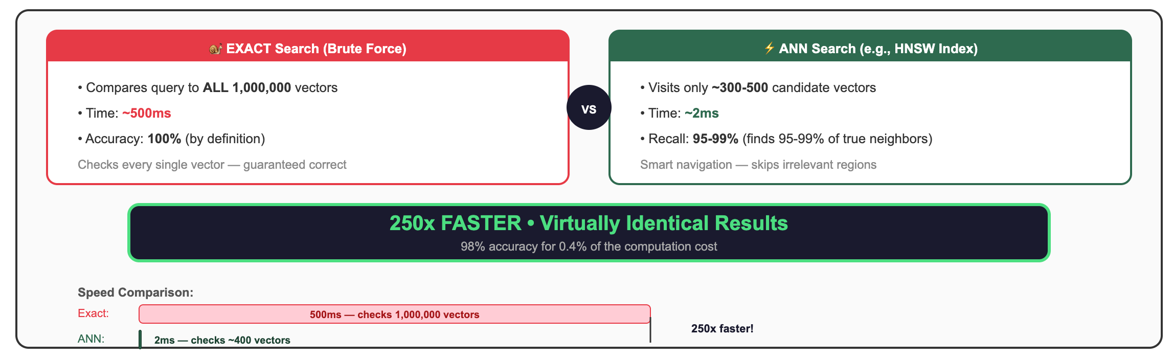
250x faster for results that are 98% as accurate. In RAG, where the LLM can work with any of several relevant documents, this trade-off isn’t just acceptable, it’s the only sane choice.
The Trade-Off: 95-99% Recall at 100-1000x Speed
Let’s define “recall” precisely:
Recall = (Number of true nearest neighbors found by ANN) / (Total true nearest neighbors)
If you ask for the top-10 nearest neighbors:
100% recall: ANN returns the exact same 10 vectors as brute-force would
95% recall: ANN returns 9 or 10 of the correct vectors (maybe swaps one for a slightly-less-similar alternative)
90% recall: ANN returns 9 of the correct vectors
Most modern ANN implementations achieve 95-99% recall while being 100-1000x faster than exact search. And here’s the beautiful part: you can usually tune this trade-off. If you need a higher recall, the algorithm searches a bit more broadly (slightly slower). If you need more speed, it searches more aggressively (slightly lower recall).
For RAG applications, 95% recall is almost always sufficient. Here’s the deeper reasoning:
You’re retrieving multiple documents (top-5, top-10), so missing one rarely matters. The LLM synthesizes information across all retrieved chunks. If one chunk is swapped for a slightly-less-relevant alternative, the final answer is virtually identical.
The LLM is robust to imperfect context. Large language models don’t need the single perfect document, they can extract relevant information from documents that are “pretty good.” The difference between similarity scores of 0.93 and 0.91 is imperceptible to the model.
The difference between the 5th and 6th most similar document is usually negligible. Similarity scores in the top results tend to cluster together. The gap between rank 1 and rank 10 might be 0.94 vs 0.89, both highly relevant.
Users care about response time. 12ms vs 3,200ms is the difference between “snappy” and “did the app crash?” In user studies, response latency above 1 second significantly increases abandonment rates.
Embedding models themselves are approximate. The embedding of your query is already an imperfect representation of the user’s intent. Obsessing over the exact nearest neighbor to an approximate query vector is false precision.
Why Your RAG User Will Never Notice?
Let’s drive this home with numbers:
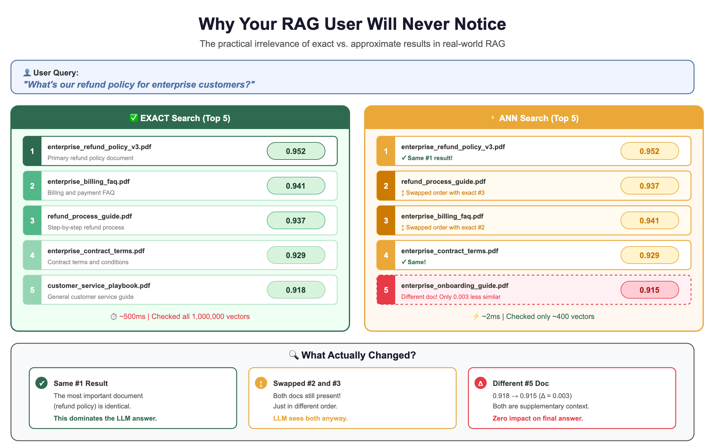
The LLM doesn’t care whether the 5th document scores 0.918 or 0.915. It’s pulling the key information from the top 1-2 results anyway.
Families of ANN Algorithms: A Brief Tour
So how do ANN algorithms achieve this magic? How do they find near-neighbors without checking everything?
The fundamental insight shared by all ANN algorithms is:
Pre-organize vectors during index building so that similar vectors can be found quickly during search, without examining every vector.
Different algorithms use different clever tricks to achieve this organization. Here’s a brief introduction to the four main families.
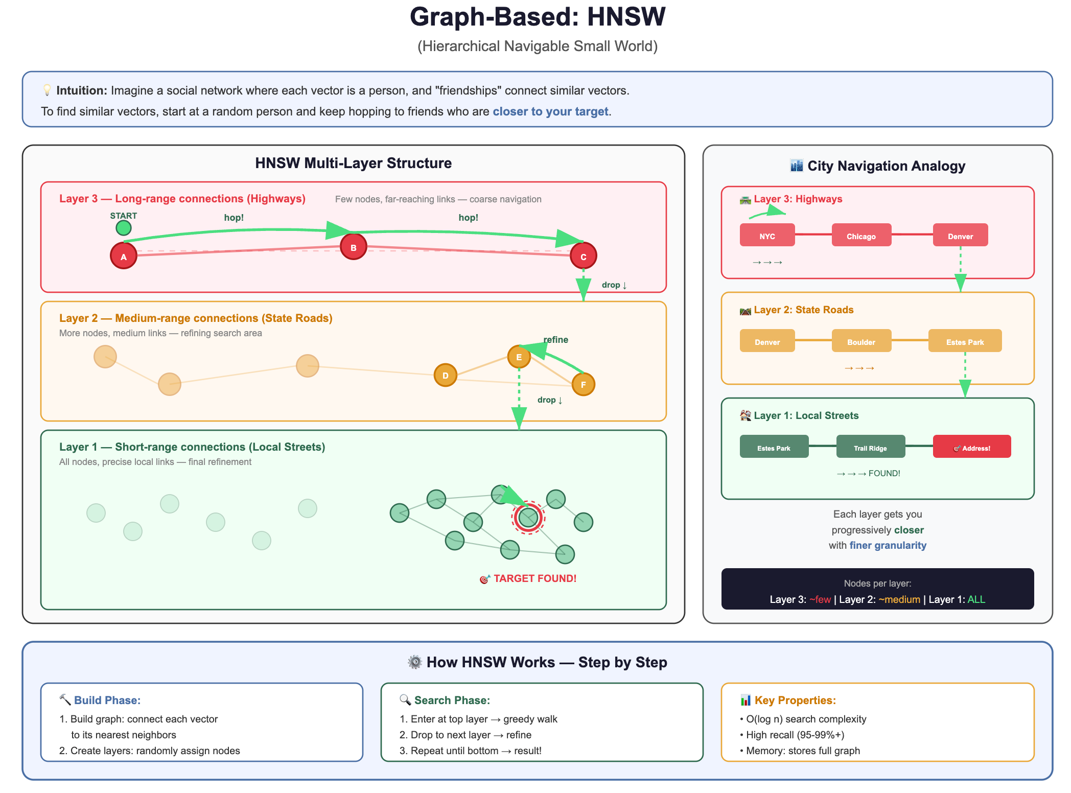
1. Graph-Based: HNSW (Hierarchical Navigable Small World)
The intuition: Imagine a social network where each vector is a person, and “friendships” connect similar vectors. To find vectors similar to your query, you start at a random person and keep hopping to their friends who are closer to your target.
How it actually works, step by step:
Building the graph: When you insert a vector, you connect it to its nearest existing neighbors (typically 16-64 connections per vector). This creates a graph where similar vectors are linked.
The “hierarchical” part: HNSW builds multiple layers, like an express train system:
Top layer: Very few vectors, connected by long-range links (like express trains between cities)
Middle layers: More vectors, medium-range links (like regional trains)
Bottom layer: All vectors, short-range links (like local buses)
Searching: Start at the top layer, greedily hop to the node closest to your query. Drop down a layer. Repeat. By the time you reach the bottom layer, you’re already in the right neighborhood, then you do a fine-grained local search.
Why it’s popular: Extremely fast queries, excellent recall, works well in practice. It’s the default choice for most vector databases today.
Trade-off: Uses more memory (stores the graph structure) and building the index is slower.
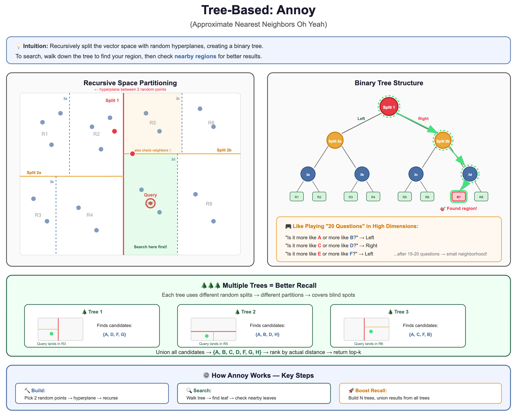
2. Tree-Based: Annoy (Approximate Nearest Neighbors Oh Yeah)
The intuition: Recursively split the vector space with random hyperplanes, creating a binary tree. To search, walk down the tree to find your region, then check nearby regions.
Why it’s used: Simple to understand, fast to build, memory-mappable (great for read-heavy workloads).
Trade-off: Lower recall than HNSW for the same speed. Better for static datasets.
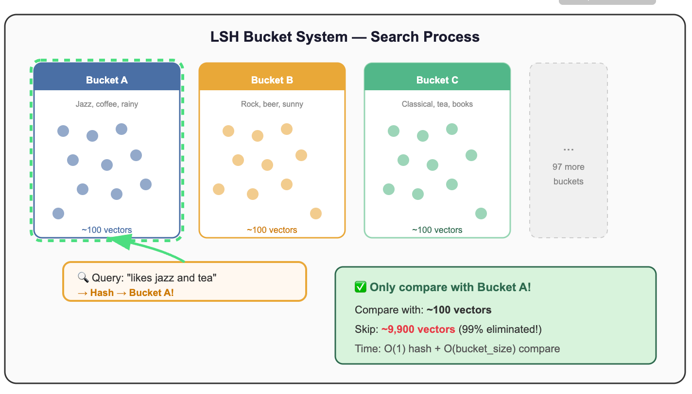
3. Hash-Based: LSH (Locality-Sensitive Hashing)
The intuition: Design hash functions where similar vectors are likely to hash to the same bucket. Then only compare vectors within the same bucket.
Why it’s used: Theoretically elegant, sub-linear query time guarantees, works well for very high-dimensional data.
Trade-off: Requires many hash tables for good recall, can use significant memory, harder to tune.
4. Quantization-Based: IVF (Inverted File Index) and PQ (Product Quantization)
The intuition: Cluster vectors into groups (like zip codes), then only search the most relevant clusters. Optionally, compress vectors to save memory.
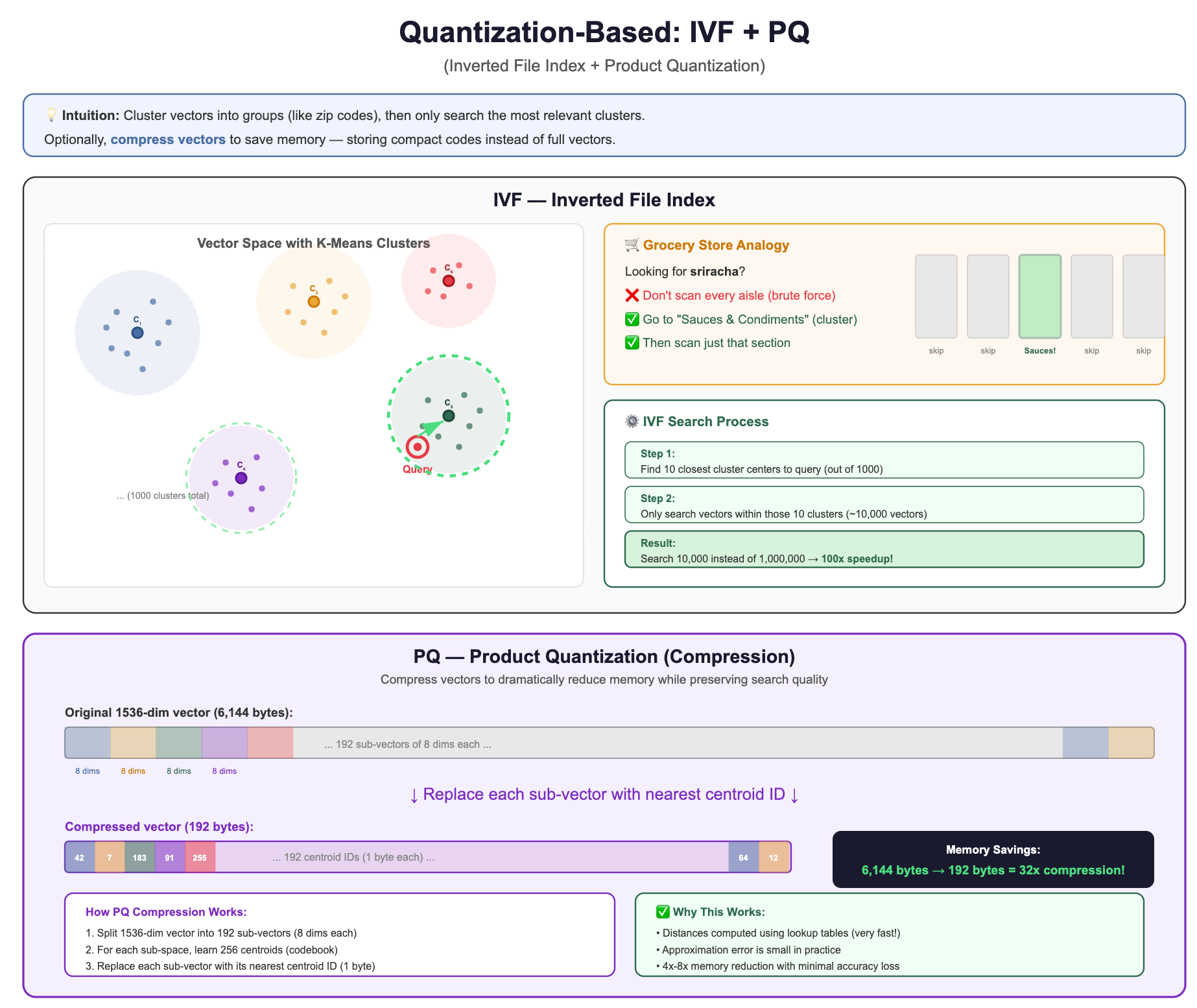
Why it’s used: Excellent memory efficiency, scales to billions of vectors, good for disk-based systems.
Trade-off: Requires training (clustering step), lower recall than HNSW at the same speed, but uses far less memory.
Comparing the Families at a Glance
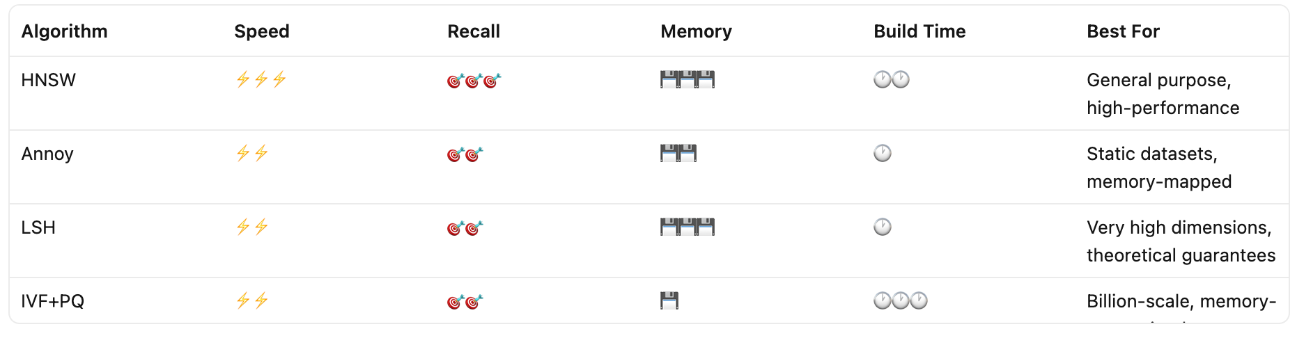
Putting It All Together
Let’s recap the journey we’ve taken in this section:
The fundamental shift:
The question changed — from “find exact matches” to “find similar things”
Traditional indexes broke — B-trees can’t partition 1,536-dimensional space
Brute force is too slow — 3 billion operations per query doesn’t scale
ANN saves the day — clever data structures find 98% of true neighbors in 0.1% of the time
“Approximate” is a feature, not a bug — for RAG, close enough IS good enough
🧪 Quick Self-Check
Before moving on, make sure you can answer these:
Q1: Why can’t you add a B-tree index on a vector column and call it a day?
Because B-trees sort along ONE dimension. In 1,536 dimensions, the curse of dimensionality makes spatial partitioning useless.
Q2: What does “approximate” mean in ANN, and why is it acceptable?
ANN might miss 1-5% of true nearest neighbors, but returns results 100-1000x faster. In RAG, the LLM produces virtually identical answers from either set.
Q3: If you have 10 million vectors and need <10ms query time, can you use brute force?
No. Brute force on 10M vectors ≈ 5 seconds per query. You need an ANN index.
Q4: Which ANN family would you explore first for a general-purpose RAG application?
HNSW (graph-based). Best recall-speed trade-off for most use cases. It’s the default in Pinecone, Qdrant, Weaviate, and pgvector.
Closing Thoughts:
Now you understand why vector databases exist and what makes them fundamentally different from relational databases. In in the next lesson, we'll dive into the storage architecture beneath the vectorDB, where decisions about sharding, replication, and persistence determine whether your RAG system thrives under production load or crumbles when real users show up.