
Lesson 4.2 : How Does an Embedding Model Work?

In Lesson 4.1, we learned that embeddings turn text into coordinates in meaning-space — where “cardiac arrest” and “heart attack” become nearby points even though they share zero words. We understood what embeddings are and why they matter for RAG. Now the natural next question: what’s actually happening inside that black box between text going in and the numbers coming out?
Let’s crack open the hood.
Here’s what we’ll cover:
The type of Transformer architecture used for embeddings (encoder vs. decoder)
How text becomes numbers (tokenization)
How the model builds contextual understanding (attention)
How per-token representations collapse into a single vector (pooling)
How these models are trained to produce meaningful embeddings (training objectives)
How embedding models are used in practice for retrieval (bi-encoder vs. cross-encoder)
How to choose the right model (MTEB benchmark)
Two Kinds of Transformer
The original Transformer architecture (from the 2017 “Attention Is All You Need” paper) was designed for sequence-to-sequence tasks like machine translation. It has two parts, an encoder that reads the source sentence (e.g., English) and a decoder that generates the target sentence (e.g., French). Since then, researchers have built models using just one half or the other.
These two halves do very different jobs.
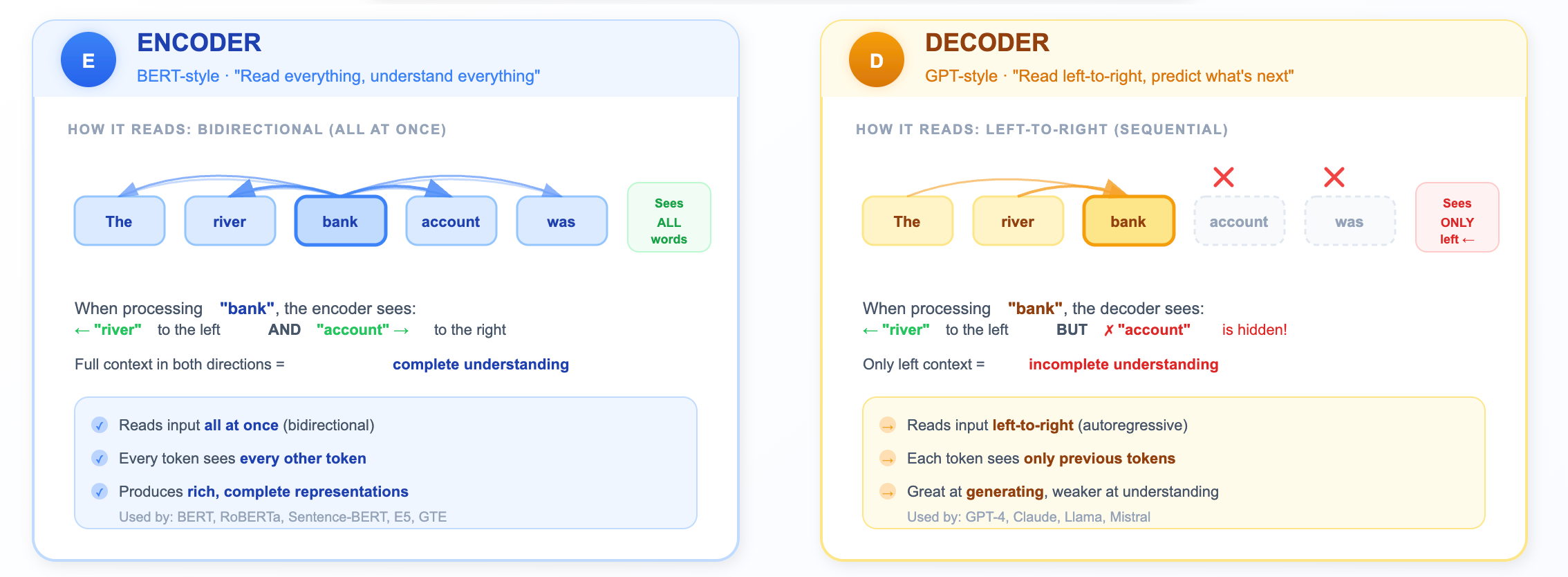
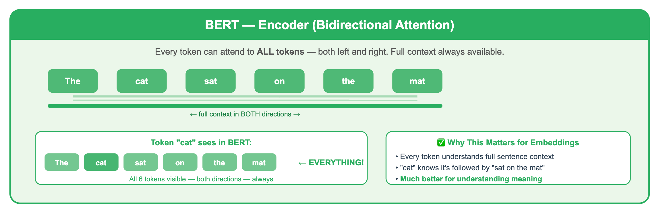
The Encoder (BERT-style): “Read everything, understand everything”
An encoder processes all tokens with full visibility. Every word is allowed to attend to every other word through the attention mechanism. When the encoder processes the word “bank,” it can look left at “river” AND right at “account” to figure out what “bank” means.
By “simultaneously,” we mean every token is allowed to attend to every other token in the attention mechanism, not that computation is literally instant. The model still does matrix math, but no token is blocked from seeing any other token.
This bidirectional view makes encoders natural understanding machines. They produce a rich representation of the entire input.
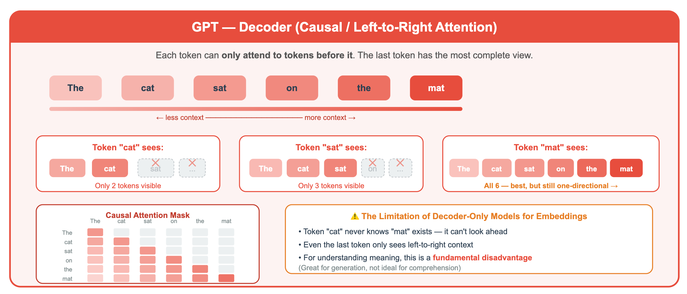
The Decoder (GPT-style): “Read left-to-right, predict what’s next”
A decoder processes tokens sequentially. Each token can only see the tokens that came before it (enforced by a “causal mask” in the attention mechanism). When GPT encounters “bank,” it can see “river” if it came earlier, but it cannot peek ahead at “account.”
This left-to-right constraint exists for a reason, it’s what makes GPT great at generating the next word. You can’t predict the next word if you’ve already seen it! But it means the representation of any given token is incomplete. It’s always missing context from the right.
Why do decoders exist if encoders are better at understanding? Because understanding and generation are different tasks. If you want to generate text (chatbots, writing assistants, code completion), you need the left-to-right constraint, it’s what allows the model to produce one token at a time. Encoders are great at understanding existing text; decoders are great at creating new text.
Why This Matters for Embeddings?
An embedding is supposed to capture the full meaning of a piece of text. You need the model to have seen all of it. Encoders do this naturally. Decoders... don’t.
That’s why embedding models are overwhelmingly encoder-based (BERT-style).
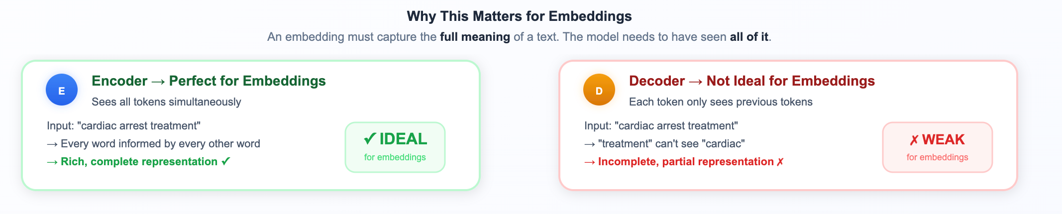
Why this matters for RAG specifically: When your RAG system encodes a document chunk about "staff retention strategies," the encoder sees all those words together and produces a vector that captures the full meaning. Later, when a user asks about "reducing employee turnover," the encoder produces a nearby vector, because it understood both complete phrases. This bidirectional understanding is what makes semantic matching possible.
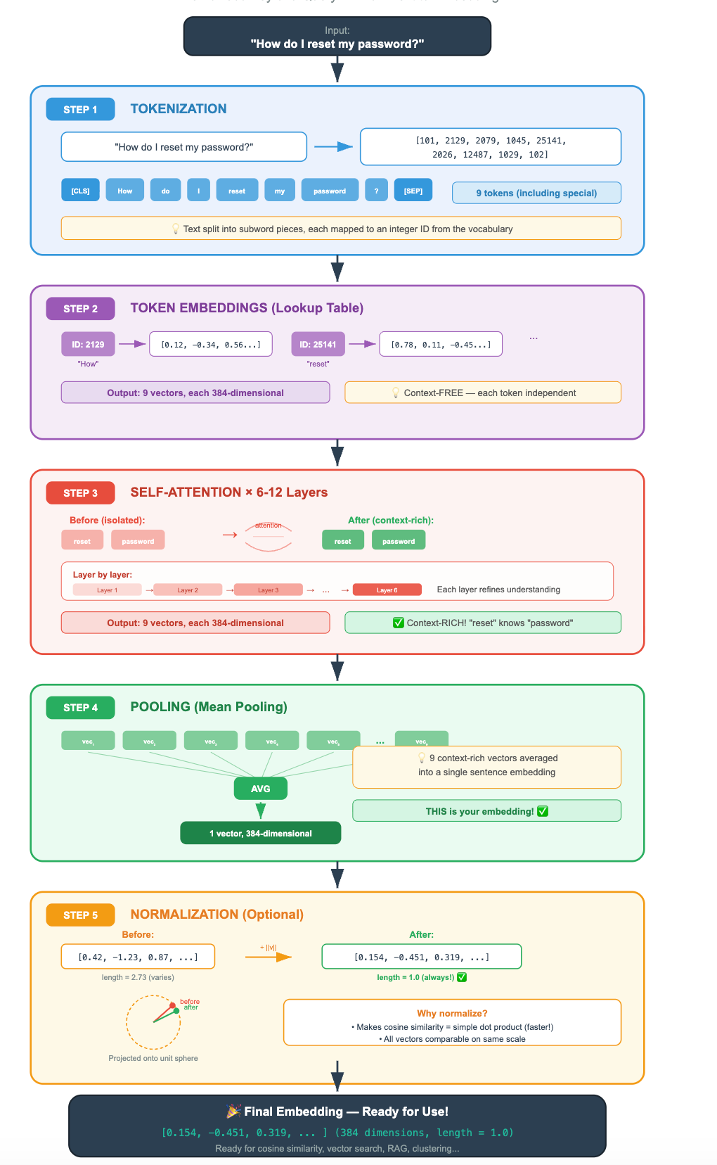
Tokenization
Before any transformer magic happens, your text needs to become numbers. Models don’t read English, they read numbers
The Problem with Whole Words
You might think: “Just assign each word a number.” But what about:
“unhappiness” — should that be one token or three? (
un+happi+ness)“ChatGPT” — this word didn’t exist when most models were trained
“pneumonoultramicroscopicsilicovolcanoconiosis” — good luck with that one
Modern models use subword tokenizers (like WordPiece or BPE) that break text into frequently occurring pieces:
The core idea behind BPE: Start with individual characters as your vocabulary. Then iteratively scan a massive text corpus and merge the most frequently adjacent pair of tokens into a new single token. Repeat thousands of times. After training:
Very common words like “the,” “is,” “and” remain as whole tokens (they were merged early and often)
Less common words get split into recognizable pieces: “unhappiness” → “un” + “##happi” + “##ness”
Rare or novel words get split into smaller pieces, sometimes down to individual characters
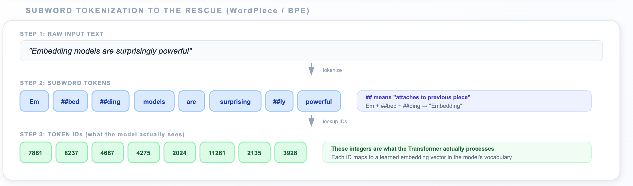
The ## prefix means “this piece attaches to the previous one.” The tokenizer learned these pieces from a massive corpus where the common words stay whole, rare words get split.
📝 Note: Every model has its own tokenizer with its own vocabulary. You can’t mix tokenizers between models. When you load
sentence-transformers/all-MiniLM-L6-v2, the correct tokenizer comes bundled with it.
Special Tokens
The tokenizer also adds bookkeeping tokens that the model expects:
[CLS]— “Classification” token, placed at the start. Acts as a summary position.[SEP]— “Separator” token, marks the end of the input (or separates two inputs).c
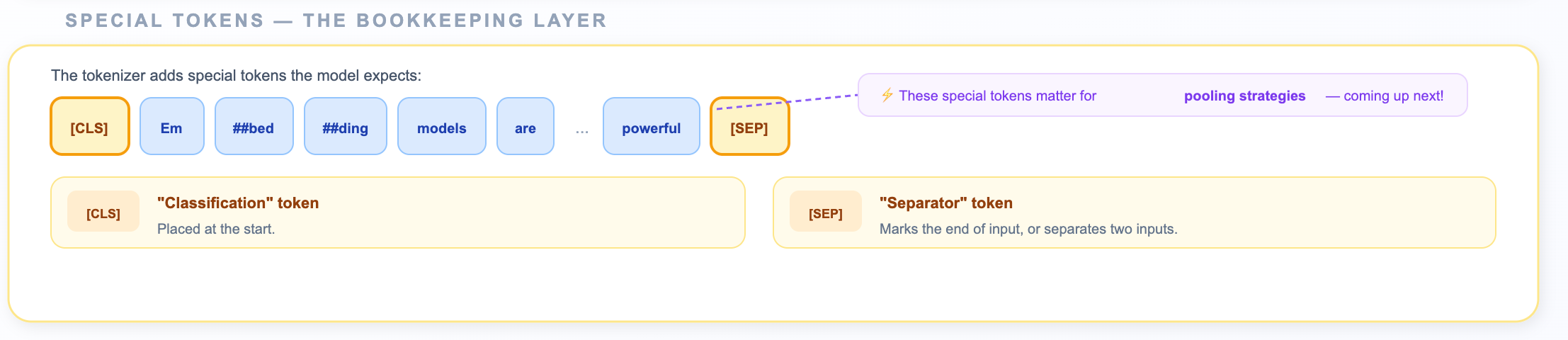
These tokens will matter a lot when we talk about pooling strategies in a few minutes.
Attention — The Secret Sauce
After tokenization, each token ID gets mapped to an initial vector (from a learned lookup table). These initial vectors are context-free, the vector for “bank” is the same whether it appears after “river” or “savings.”
Then the Transformer’s self-attention mechanism kicks in.
Self-attention lets every token ask: “Which other tokens in this sentence should I pay attention to in order to understand myself better?”
How Attention Actually Works?
Here’s the intuition behind the mechanism. Each token generates three vectors:
Query (Q): “What am I looking for?” — represents what information this token needs
Key (K): “What do I contain?” — represents what information this token can offer
Value (V): “What information do I carry?” — the actual content to be passed along
The process works like this:
Each token’s Query is compared against every other token’s Key (via dot product)
High Query-Key similarity = high attention score (”these two tokens are relevant to each other”)
These scores become weights (after softmax normalization)
Each token’s new representation = weighted sum of all tokens’ Values\
Let’s watch it work:

After attention, the vector for “bank” is different in these two sentences. The same word, the same initial token ID, but completely different output vectors. This is what makes contextual embeddings so powerful compared to older approaches like Word2Vec.
Multiple Layers of Attention
The model doesn’t just run one attention pattern, it runs several in parallel (typically 8 or 12), called “heads.” Each head can learn to focus on different types of relationships:
One head might track syntactic relationships (subject-verb agreement)
Another might track coreference (”it” refers to “the company”)
Another might track semantic similarity (synonyms and related concepts)
The outputs of all heads are concatenated and combined, giving each token a rich, multi-faceted representation.
A typical embedding model has 6 to 12 layers of attention stacked on top of each other. Each layer refines the representations further:
Example:
Layer 1: Basic syntax — “bank” is a noun
Layer 2: Local context — “bank” is near “river”
Layer 3: Broader patterns — this is a nature scene
...
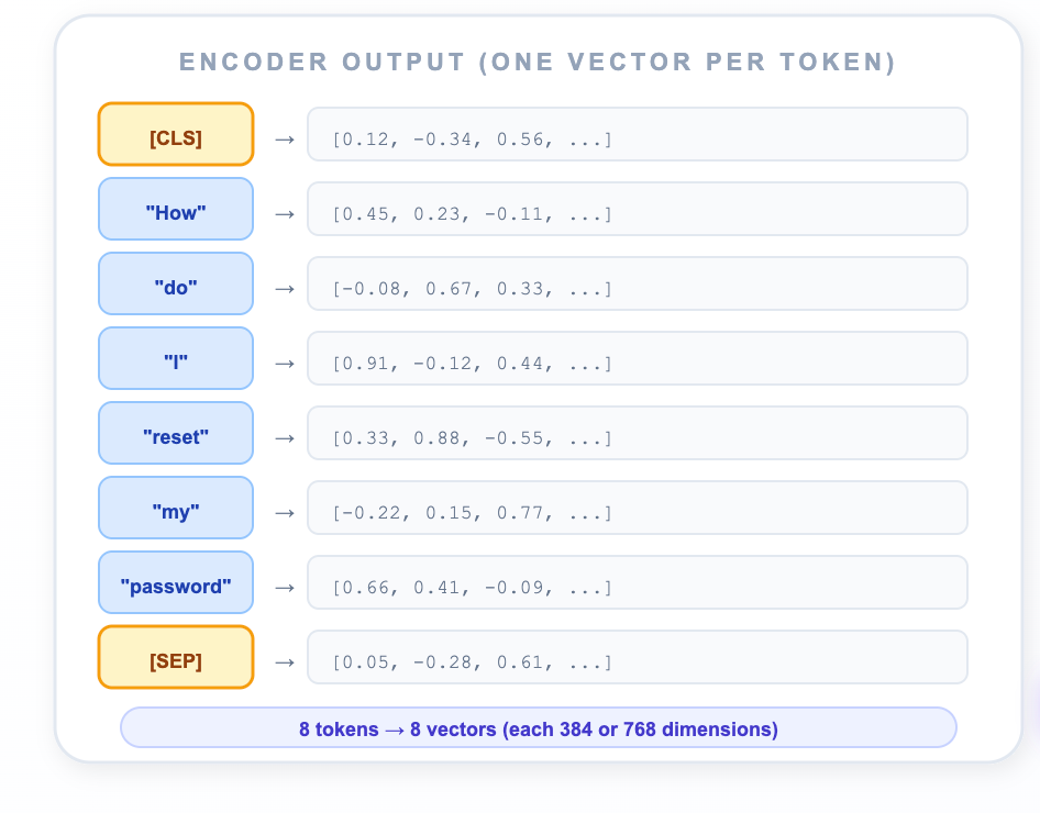
Layer 12: Rich semantic meaning — full contextual understandingAfter all layers, you have one refined vector per token. For a 10-token input, you have 10 vectors. But you need one vector for the whole text.
Why this matters for RAG: This contextual understanding is why your RAG system can match a query about “reducing employee turnover” with a document about “staff retention strategies”, the embedding model understands they mean the same thing, even though they share zero words. The attention mechanism has learned that “turnover” in an HR context and “retention” are semantically related.
That's where pooling comes in.
Pooling — From Many Vectors to One
The encoder gives you a matrix of vectors, one per token. But for retrieval, you need a single vector that represents the entire input. The strategy for collapsing these vectors is called pooling.
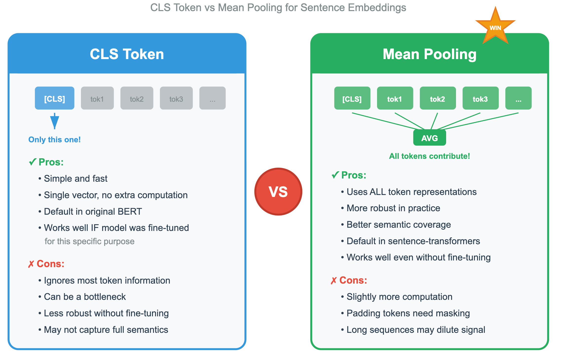
Strategy 1: CLS Token Pooling
In CLS Token pooling, just take the vector from the [CLS] token and use it as the sentence embedding.
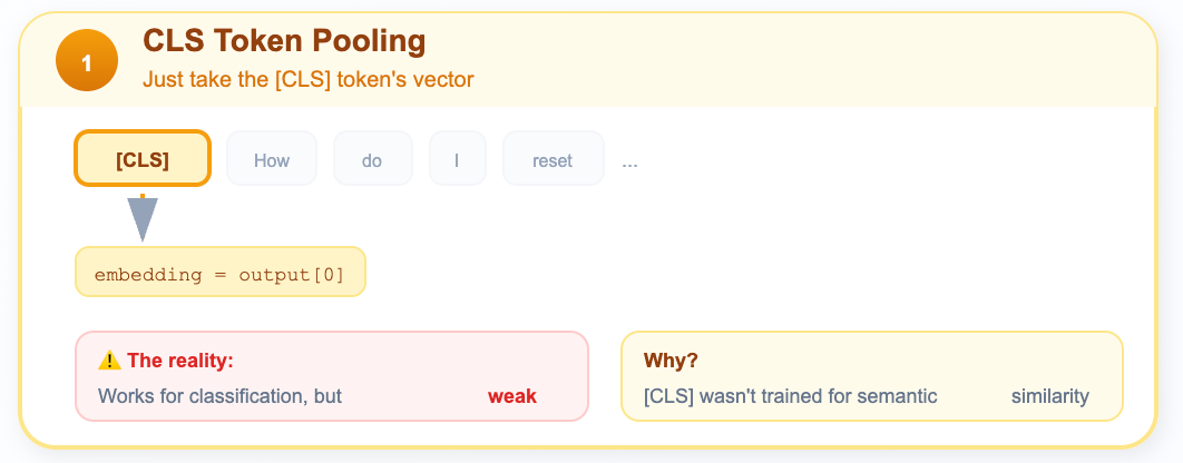
During BERT’s pre-training, the [CLS] token was used for the “Next Sentence Prediction” task, so it should have learned to aggregate sentence-level meaning.
In reality it works okay for classification tasks, but for semantic similarity, it’s actually pretty bad out of the box. The [CLS] token wasn’t explicitly trained to capture semantic meaning for retrieval.
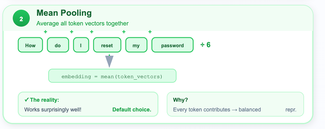
Strategy 2: Mean Pooling
In mean pooling, we average all the token vectors together (excluding padding tokens).
Example:
# Mean pooling — the workhorse
# Mask out padding tokens, then average
token_vectors = encoder_output[1:-1]  # Skip [CLS] and [SEP]
sentence_embedding = mean(token_vectors)
Every token contributes to the overall meaning. Averaging them gives a balanced representation.
In reality this works surprisingly well! And it’s the default strategy for most modern sentence embedding models.
Which strategy Wins?
Practical Tip: You almost never implement pooling yourself. When you use a library like
sentence-transformers, the pooling strategy is baked into the model configuration. But understanding it helps you debug weird results, like when someone accidentally uses raw BERT with CLS pooling and wonders why their retrieval is terrible.
Bi-Encoder vs. Cross-Encoder
Now here’s where things get really interesting for RAG. There are two fundamentally different ways to use Transformer encoders for comparing a query to a document.
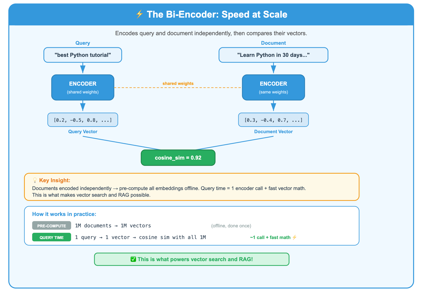
The Bi-Encoder:
A bi-encoder encodes the query and the document independently, then compares their vectors.
Because query and document are encoded independently, you can pre-compute all document embeddings ahead of time. At query time, you only encode the query (one forward pass) and then do fast vector math.
This is what makes vector search possible. This is what you use in RAG.
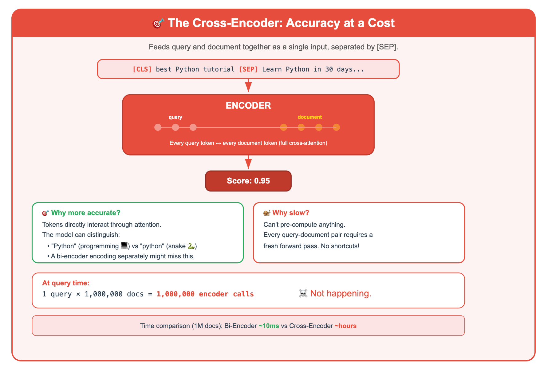
The Cross-Encoder:
A cross-encoder feeds the query and document together as a single input, separated by a [SEP] token.
Why is this more accurate? Because the query and document tokens can directly interact through attention. The model can notice that the query says “Python” and the document says “python” (the snake), and it can figure out they’re talking about different things. A bi-encoder, encoding them separately, might miss this nuance.
But this is slow, because you can’t pre-compute anything. Every query-document pair requires a fresh forward pass through the encoder.
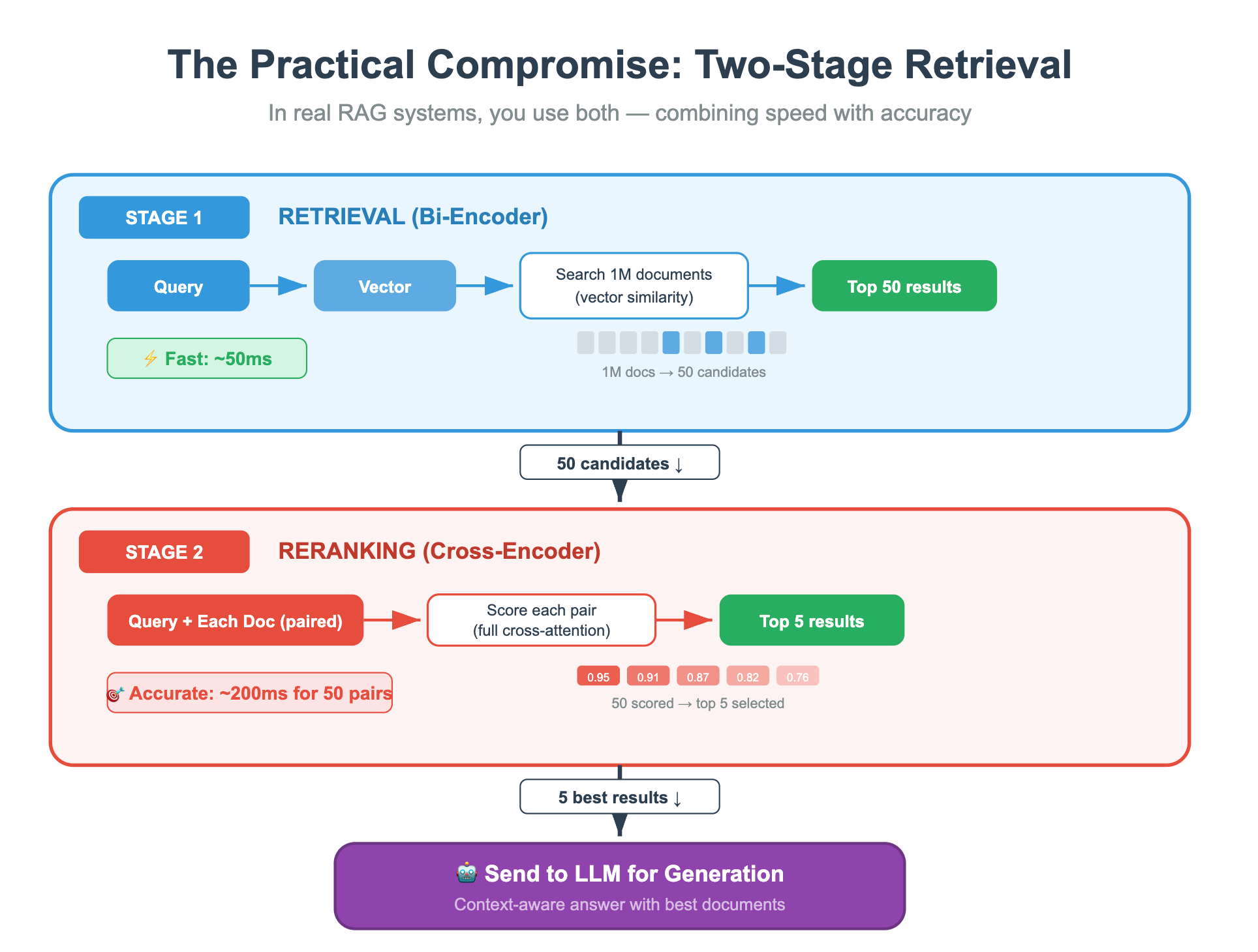
The Practical Compromise: Two-Stage Retrieval
In real RAG systems, you use both. This pattern is called "retrieve and rerank":
Think of it like hiring. The bi-encoder is the resume screening software that quickly filters 10,000 applicants down to 50. The cross-encoder is the hiring manager who carefully reads those 50 resumes and picks the top 5 for interviews. You’d never ask the hiring manager to read all 10,000 resumes. And you’d never let the screening software make the final hire.
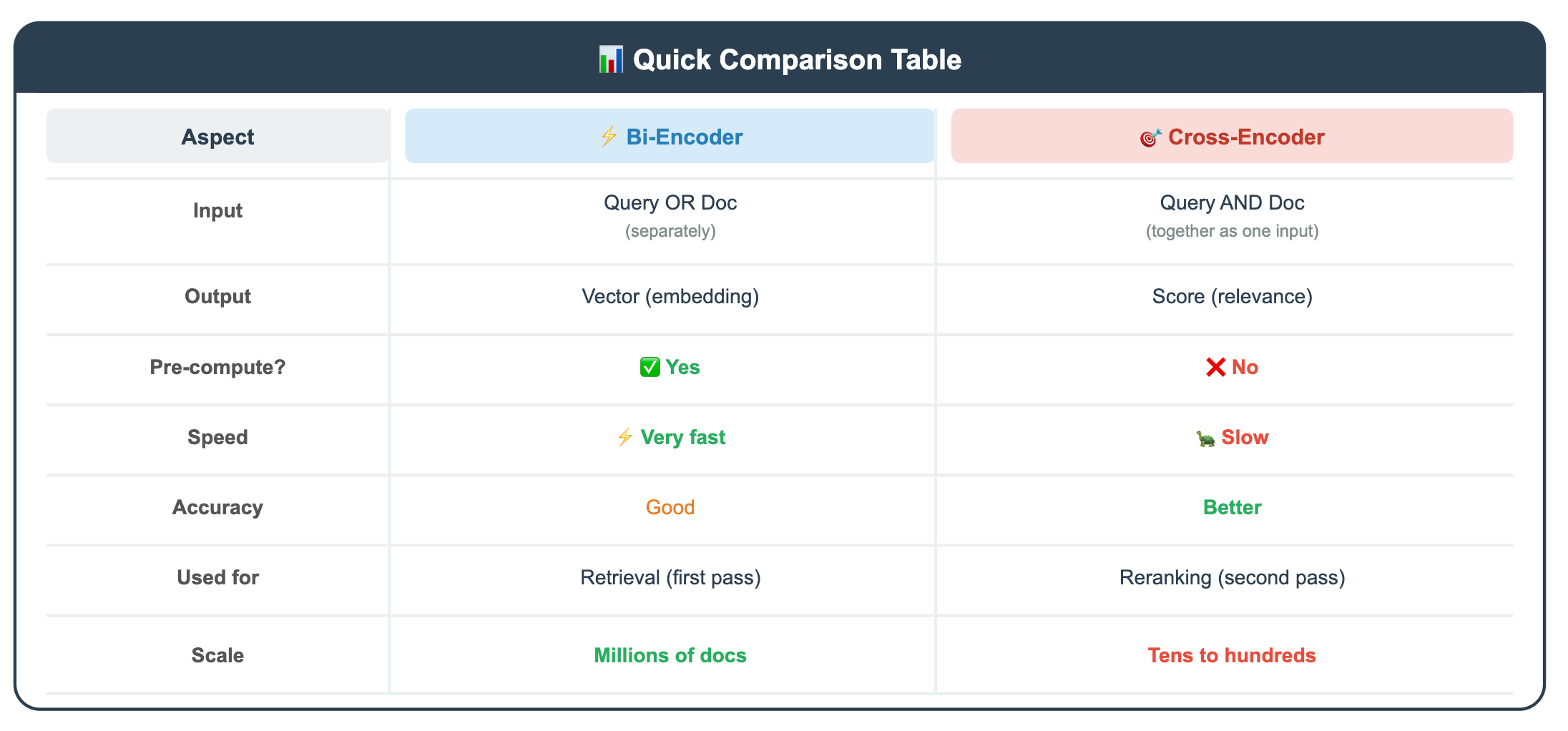
Here’s a quick comparison table:
So, Why You Can’t Just Use GPT as an Embedding Model
You might wonder, “GPT is huge and powerful. Can’t I just take the hidden states from GPT and use those as embeddings?”
You can, but there are some real problems:
Problem 1: The Causal Attention Mask
GPT is a decoder. Each token can only attend to tokens before it. The last token has the most complete view, but even it has only seen the text in one direction.
Problem 2: Trained for Generation, Not Representation
GPT was trained to predict the next token. Its internal representations are optimized for “what word comes next?” and not “what does this whole passage mean?” Using raw GPT hidden states for similarity search gives mediocre results.
Problem 3: It’s Expensive
GPT models are enormous. Encoding every document in your knowledge base through a 175B-parameter model is orders of magnitude more expensive than using a purpose-built 110M-parameter embedding model.
The Exception: Modified Decoders
Some recent models do use decoder architectures for embeddings, but with modifications:
Removing the causal mask so tokens can attend in both directions
Adding contrastive training so the model learns to produce meaningful sentence representations
Using special pooling (like taking the last token’s representation with a special
[EOS]token)
Examples include models like e5-mistral-7b-instruct and SFR-Embedding-Mistral. These are effective but much larger and slower than BERT-style models.
Key Takeaway: It’s not that decoders can’t produce embeddings. It’s that they weren’t designed for it, and making them work requires significant architectural and training modifications. For most RAG applications, a well-trained BERT-style bi-encoder is the right tool.
How Do You Know Which Model Is Best?
You’ve decided you need a bi-encoder embedding model. You go to Hugging Face and find... hundreds of them. How do you choose?
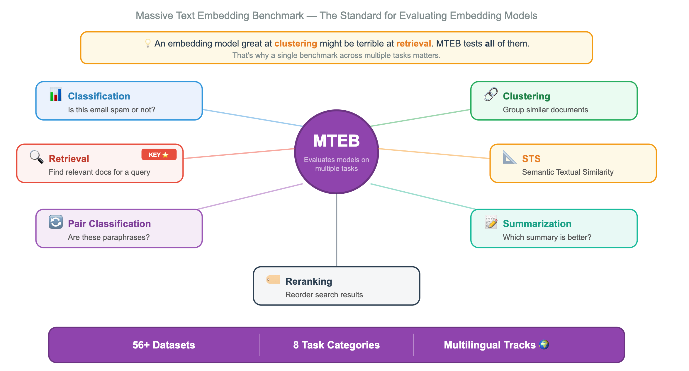
This is where a benchmark would be of great help. MTEB: Massive Text Embedding Benchmark allows you to find the right embedding model.
What Is MTEB?
MTEB is a standardized benchmark that evaluates embedding models across multiple tasks, not just one. This matters because an embedding model that’s great at clustering might be terrible at retrieval.
How to Read the MTEB Leaderboard?
You can find it at huggingface.co/spaces/mteb/leaderboard. Here’s what to look for:
Example:
┌──────────────────────┬──────────┬───────────┬───────────┬──────────┐
│ Model                │ Avg Score│ Retrieval │ Size (M)  │ Dim      │
├──────────────────────┼──────────┼───────────┼───────────┼──────────┤
│ voyage-3             │  67.3    │  72.1     │  ???      │ 1024     │
│ text-embedding-3-lg  │  64.6    │  69.8     │  ???      │ 3072     │
│ bge-large-en-v1.5    │  64.2    │  68.4     │  335      │ 1024     │
│ all-MiniLM-L6-v2     │  56.3    │  49.5     │  22       │ 384      │
│ ...                  │          │           │           │          │
└──────────────────────┴──────────┴───────────┴───────────┴──────────┘
         (Illustrative — check the live leaderboard for current numbers)
What to Actually Care About for RAG
Here’s the thing most people get wrong: don’t just sort by average score. For RAG, you care about specific columns:
Example:
Building a RAG system?
  → Look at the RETRIEVAL score (nDCG@10 on datasets like MS MARCO, NFCorpus, etc.)

Building a semantic search deduplication tool?
  → Look at the STS score

Building a document classifier?
  → Look at the CLASSIFICATION score

The “average” score blends all tasks — a model could rank #1 overall
but be mediocre at retrieval specifically.
The Tradeoffs You’ll See on MTEB
As you scan the leaderboard, you’ll notice clear patterns:
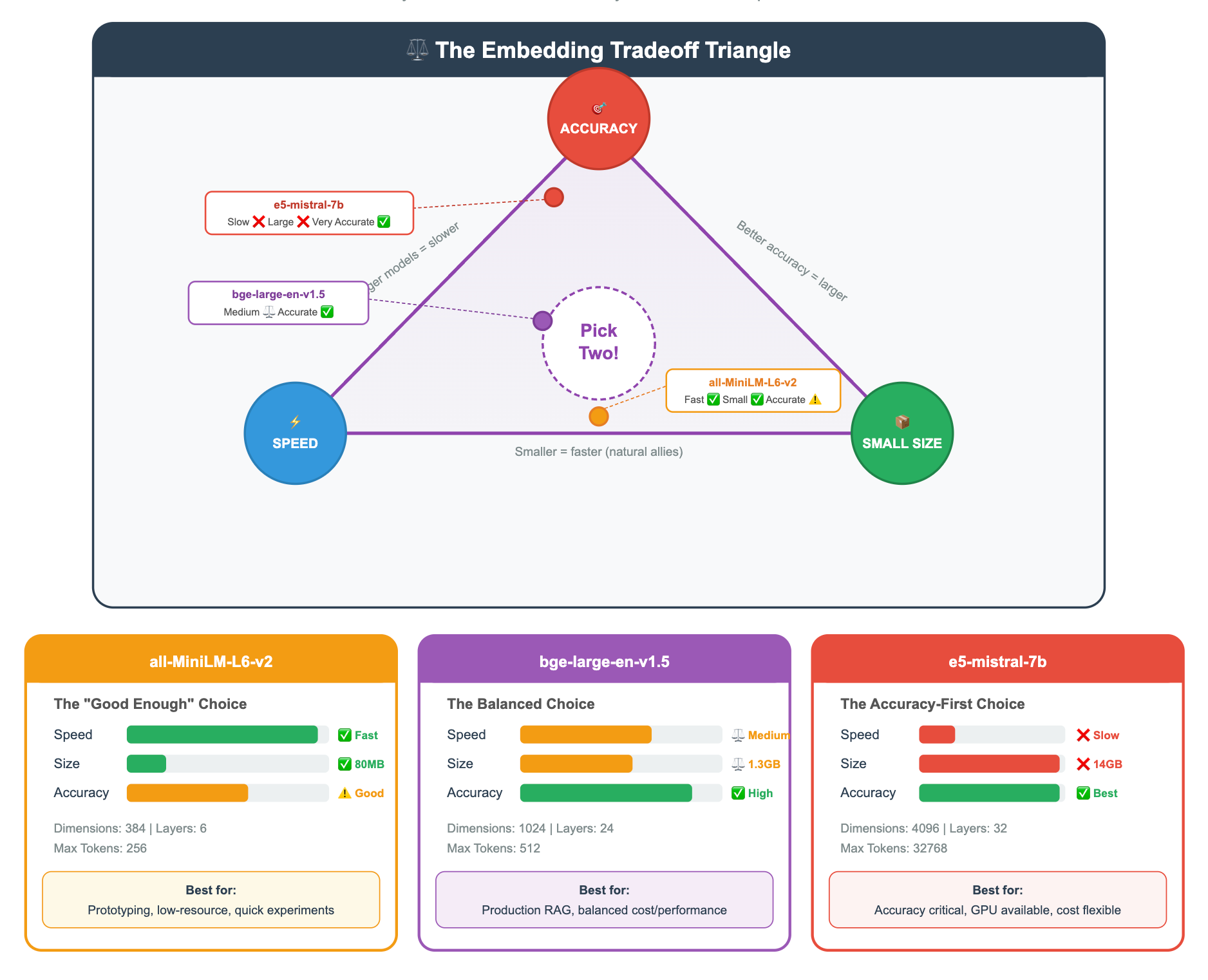
Practical Tip: For most RAG prototypes, start with a mid-range model like
bge-base-en-v1.5orall-MiniLM-L6-v2. They’re fast, small enough to run on a laptop, and good enough to validate your pipeline. Upgrade to a larger model only when you’ve confirmed that embedding quality (not chunking, not prompting, not something else) is your bottleneck.
Putting It All Together: The Full Journey of a Query
Let’s trace the complete path from text to embedding, now that you understand every step:
🧪 Check Your Understanding
Before moving on, make sure you can answer these:
1. Why does BERT produce better embeddings than GPT out of the box?
Because BERT is an encoder, it uses bidirectional attention, so every token sees the full context. GPT is a decoder with causal (left-to-right) attention, so tokens have an incomplete view.
2. You have 2 million documents and a user query. Why can’t you use a cross-encoder for retrieval?
A cross-encoder requires feeding the query AND each document together through the model. That’s 2 million forward passes per query, impossibly slow. You need a bi-encoder to pre-compute document embeddings, then compare with fast vector math.
3. Your retrieval results seem mediocre. A colleague suggests adding a cross-encoder reranker. Where in the pipeline would it go?
After the bi-encoder retrieves the top-k candidates (say, top 50), the cross-encoder re-scores those 50 query-document pairs and reorders them. You then take the top 5 from the reranked list.
4. You’re choosing an embedding model for a RAG system. On the MTEB leaderboard, Model A has a higher average score but Model B has a higher retrieval score. Which do you pick?
Model B. For RAG, retrieval performance is what matters. The average score includes tasks like classification and clustering that aren’t relevant to your use case.
You now understand the machinery of embedding from architecture to training to inference. In the next lesson, we'll get practical: given YOUR data, YOUR budget, and YOUR latency requirements, which embedding model should you actually pick? We'll cover open-source vs. API options, general vs. domain-specific models, and how to validate that your chosen model actually works for your specific use case.
📬 Enjoying this? Tomorrow’s lesson is already written and waiting.
Subscribe for FREE to get your daily brain-friendly RAG lesson, straight to your inbox, every morning.